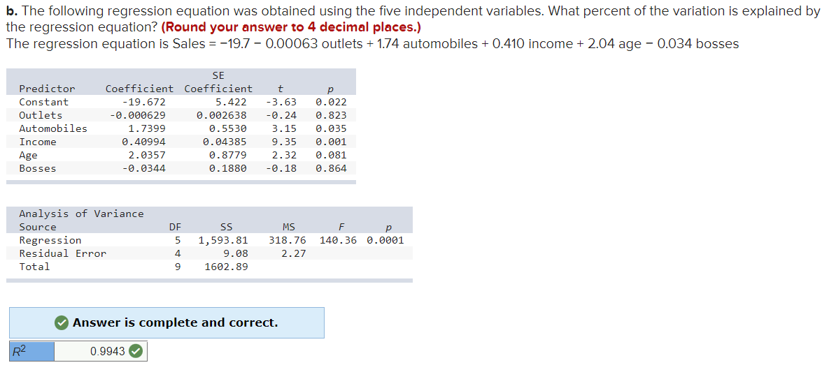
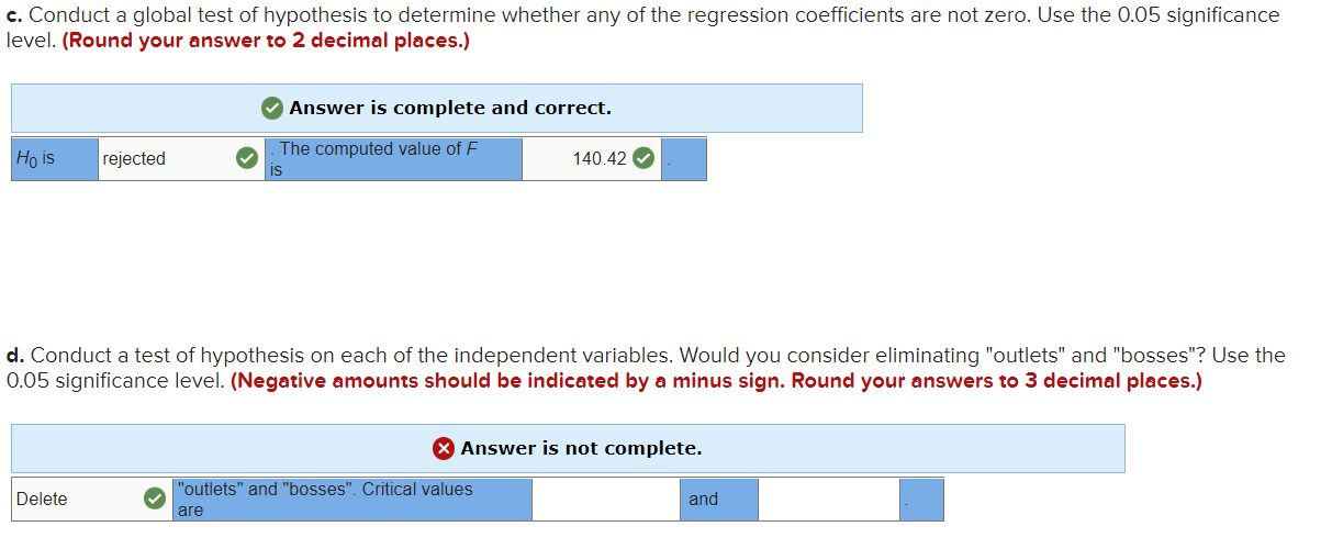
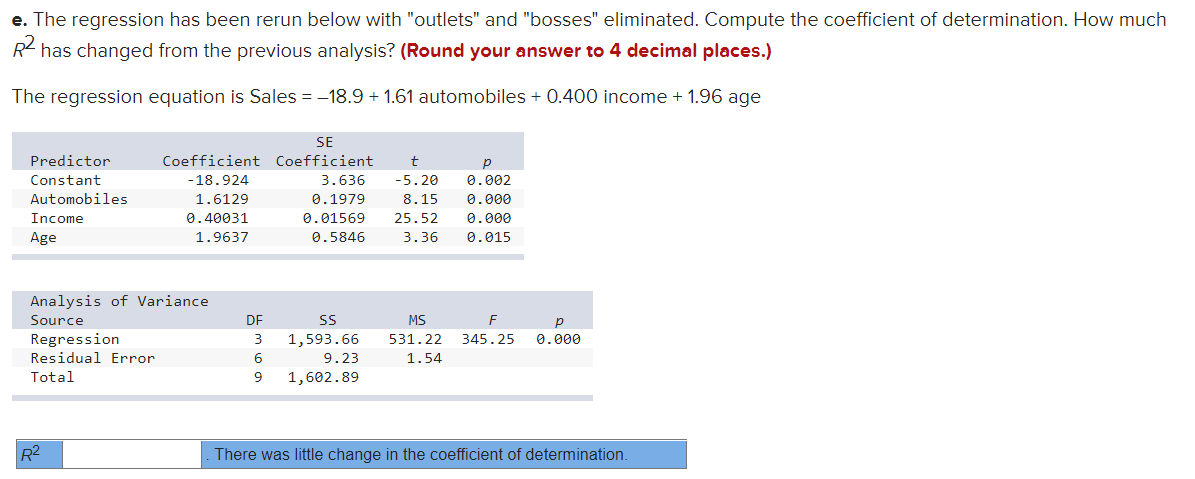
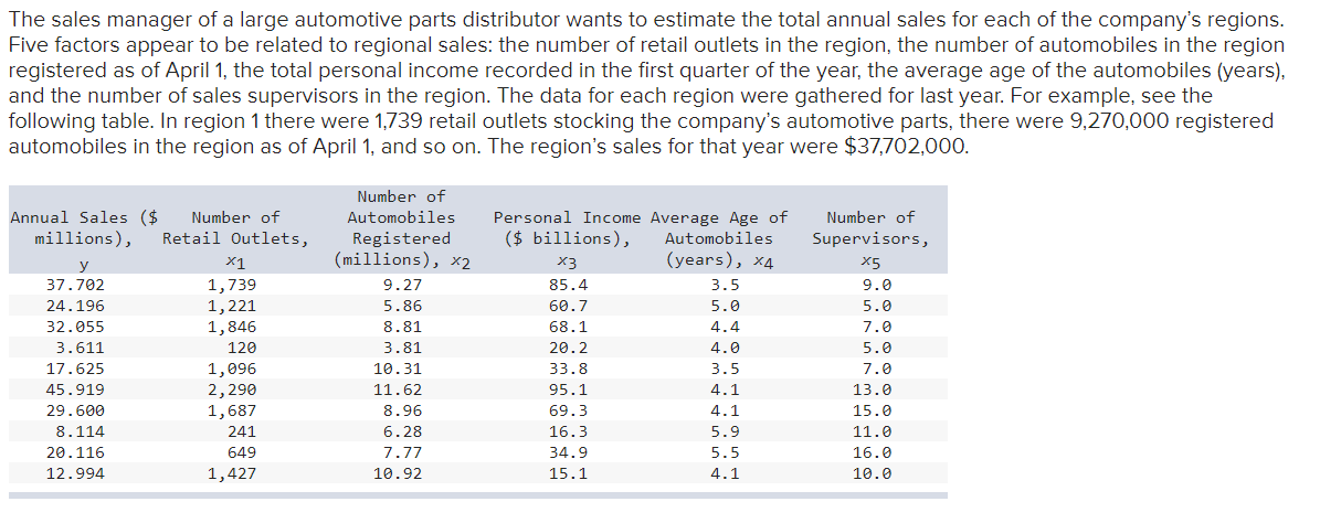
b. The following regression equation was obtained using the five independent variables. What percent of the variation is explained by the regression equation? (Round your answer to 4 decimal places.) The regression equation is Sales = -19.7 - 0.00063 outlets + 1.74 automobiles + 0.410 income + 2.04 age - 0.034 bosses SE Predictor Coefficient Coefficient t p Constant -19.672 5. 422 -3.63 0. 022 Outlets -0. 000629 0. 002638 -0. 24 0. 823 Automobiles 1. 7399 0.5530 3. 15 0. 035 Income 0. 40994 0. 04385 9. 35 0. 001 Age 2.0357 0. 8779 2. 32 0. 081 Bosses -0. 0344 0. 1880 -0. 18 0. 864 Analysis of Variance Source DF 5S MS F P Regression 5 1, 593. 81 318.76 140.36 0.0001 Residual Error 4 9. 08 2.27 Total LO 1602.89 Answer is complete and correct. R2 0.9943 Vc. Conduct a global test of hypothesis to determine whether any of the regression coefficients are not zero. Use the 0.05 significance level. (Round your answer to 2 decimal places.) 0 Answer is complete and correct. rejected 0 140.42 0 d. Conduct a test of hypothesis on each of the independent variables. Would you consider eliminating "outlets" and "bosses"? Use the 0.05 significance level. (Negative amounts should be indicated by a minus sign. Round your answers to 3 decimal places.) 9 Answer is not complete. e. The regression has been rerun below with "outlets" and "bosses" eliminated. Compute the coefficient of determination. How much R2 has changed from the previous analysis? (Round your answer to 4 decimal places.) The regression equation is Sales = 18.9 + 1.61 automobiles + 0.400 income +1.96 age SE Predictor Coefficient Coefficient f: p Constant -18.924 3.636 -5.29 9.992 Automobiles 1.6129 9.1979 8.15 9.999 Income 9.49931 9.91569 25.52 9.999 Age 1.953? 9.5846 3.36 9.915 analysis of Variance Source DF 55 MS F p Regression 3 1,593.66 531.22 345.25 9.999 Residual Error 6 9.23 1.54 Total 9 1,692.89 The sales manager of a large automotive parts distributor wants to estimate the total annual sales for each of the company's regions. Five factors appear to be related to regional sales: the number of retail outlets in the region, the number of automobiles in the region registered as of April 1, the total personal income recorded in the first quarter of the year, the average age of the automobiles (years), and the number of sales supervisors in the region. The data for each region were gathered for last year. For example see the following table. ln region 1 there were 1,739 retail outlets stocking the company's automotive parts, there were 9,270,000 registered automobiles in the region as of April1. and so on. The region's sales for that year were $37,702,000. Number of Annual Sales ($ Number of Automobiles Personal Income Average Age o'F Number of millions), Retail Outlets, Registered ($ billions), Automobiles SupervisorsJ y x1 (millions)J x2 X3 (years), X4 X5 37.792 1,739 9.27ll 85.4 3.5 9.9 24.196 1,221 5.86 68.7 5.9 5.9 32.955 1,846 8.81 68.1 4.4 2.9 3.611 129 3.81 29.2 4.9 5.9 17.625 1,996 18.31 33.8 3.5 7.9 45.919 2,299 11.62 95.1 4.1 13.9 29.699 1,68? 8.96 69.3 4.1 15.9 8.114 241 6.28 16.3 5.9 11.9 29.116 649 7.}? 34.9 5.5 16.9 12.994 1,427ll 19.92 15.1 4.1 19.9 a. Consider the following correlation matrix. Which single variable has the strongest correlation with the dependent variable? The correlations between the independent variables outlets and income and between outlets and number of automobiles are fairly strong. Could this be a problem? What is this condition called? sales outlets cars income age outlets 8 . 899 automobiles 8 . 665 8 . 775 income 8 . 964 8 . 825 8 . 489 age -8.323 8.489 -8.447 -B.349 bosses 8.286 8.183 8.395 3.155 8.291 0 Answer is complete and correct. The strongest relationship is between sales and income 0 pgblem could occur 0 if both "cars" and "outlets\" are part of the final solution Also, outlets and income are strongly correlated, This is called multicollinearity o
