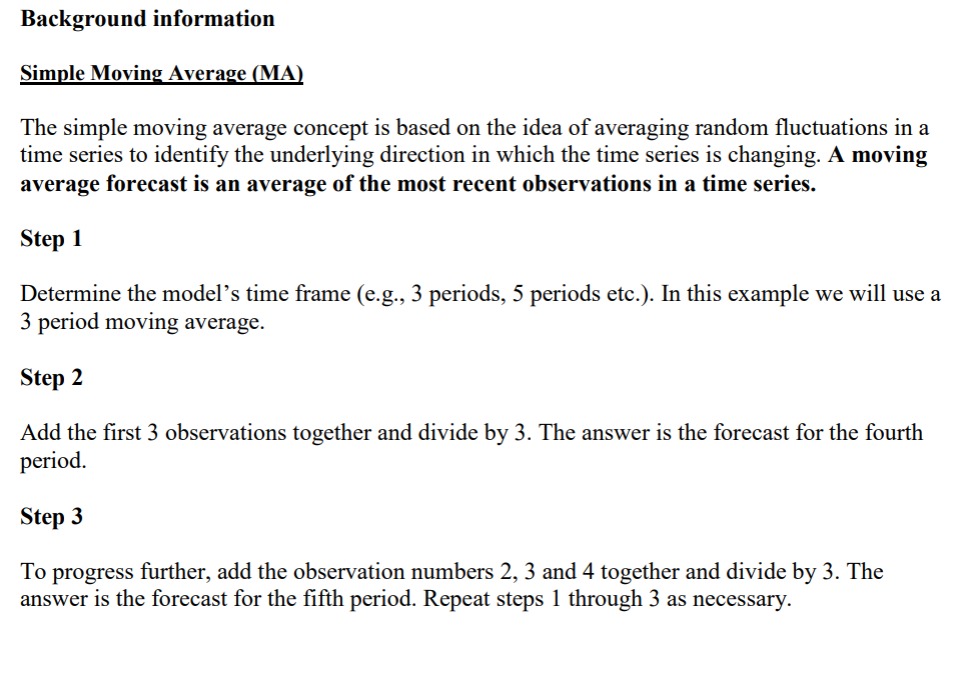
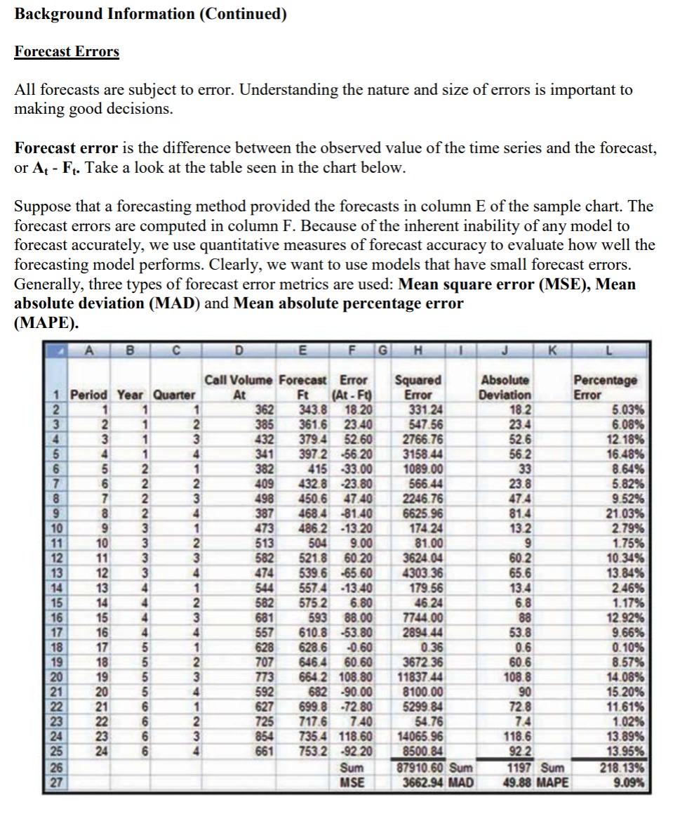
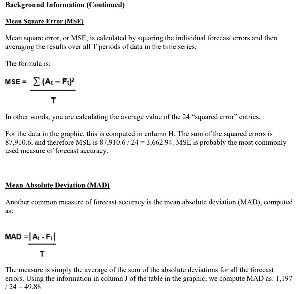
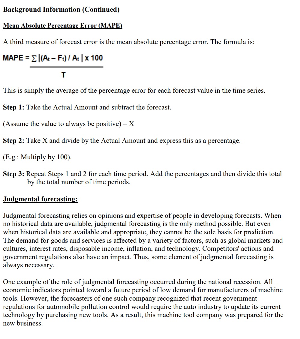
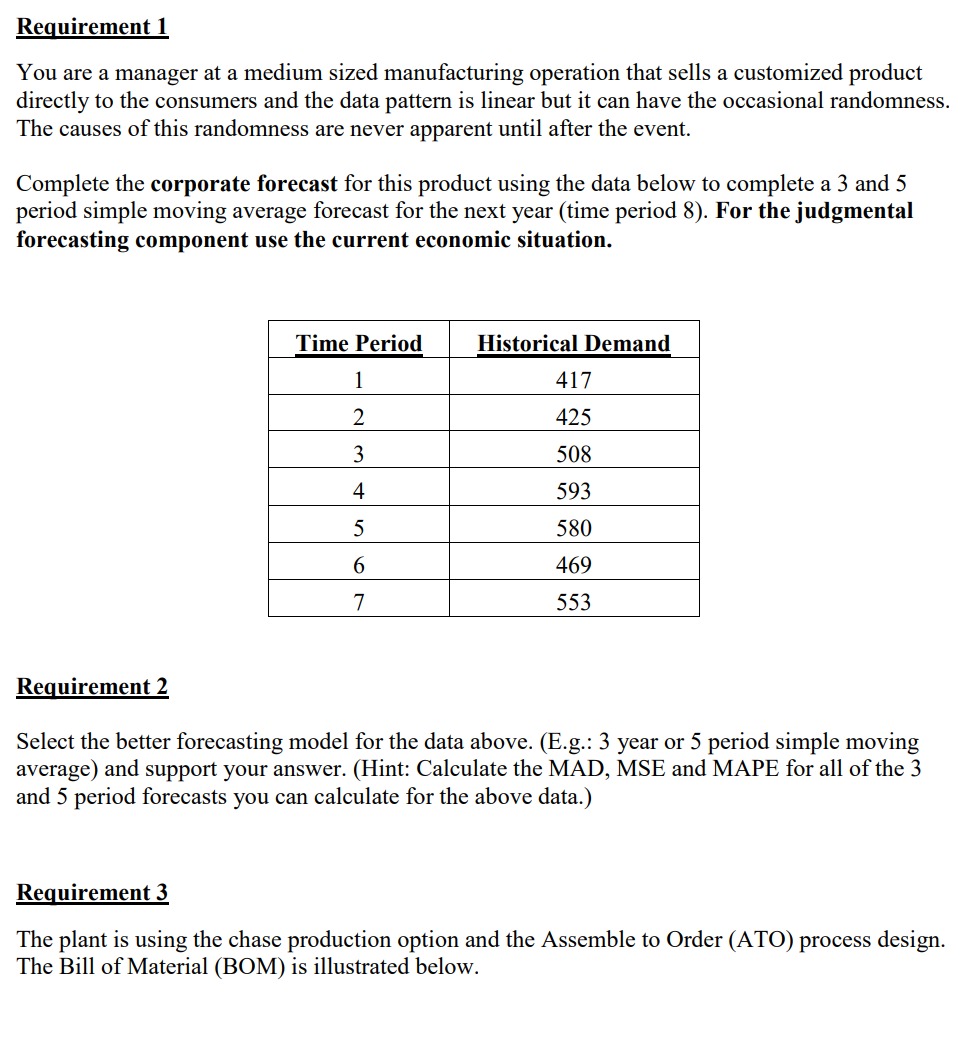
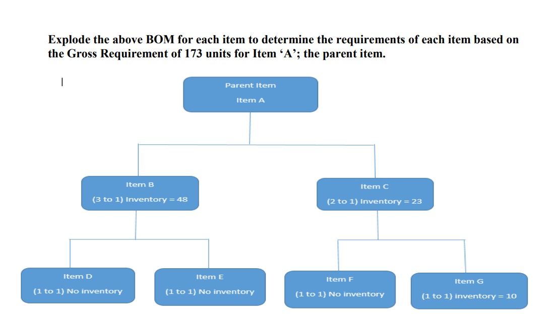
Background information Simple Moving Average (MA) The simple moving average concept is based on the idea of averaging random fluctuations in a time series to identify the underlying direction in which the time series is changing. A moving average forecast is an average of the most recent observations in a time series. Step 1 Determine the model's time frame (e.g., 3 periods, 5 periods etc.). In this example we will use a 3 period moving average. Step 2 Add the first 3 observations together and divide by 3. The answer is the forecast for the fourth period. Step 3 To progress further, add the observation numbers 2, 3 and 4 together and divide by 3. The answer is the forecast for the fifth period. Repeat steps 1 through 3 as necessary. Background Information (Continued) Forecast Errors All forecasts are subject to error. Understanding the nature and size of errors is important to making good decisions. Forecast error is the difference between the observed value of the time series and the forecast, or At Ft. Take a look at the table seen in the chart below. Suppose that a forecasting method provided the forecasts in column E of the sample chart. The forecast errors are computed in column F. Because of the inherent inability of any model to forecast accurately, we use quantitative measures of forecast accuracy to evaluate how well the forecasting model performs. Clearly, we want to use models that have small forecast errors. Generally, three types of forecast error metrics are used: Mean square error (MSE), Mean absolute deviation (MAD) and Mean absolute percentage error (MAPE). A B C D E F G H I J K L 1 Period Year Quarter Call Volume Forecast Error Squared Absolute Percentage At Ft (At-Ft) Error Deviation Error 2 1 1 1 362 343.8 18.20 331.24 18.2 5.03% 3 2 1 2 385 361.6 23.40 547.56 23.4 6.08% 4 3 1 3 432 379.4 52.60 2766.76 52.6 12.18% 5 4 1 4 341 397.2 -56.20 3158.44 56.2 16.48% 6 5 2 1 382 415 -33.00 1089.00 33 8.64% 7 6 2 2 409 432.8 -23.80 566.44 23.8 5.82% 8 7 2 3 498 450.6 47.40 2246.76 47.4 9.52% 9 8 2 4 387 468.4 -81.40 6625.96 81.4 21.03% 10 9 3 1 473 486.2 -13.20 174.24 13.2 2.79% 11 10 3 2 513 504 9.00 81.00 9 1.75% 12 11 3 3 582 521.8 60.20 3624.04 60.2 10.34% 13 14 15 16 17 18 19 20 21 22 23 24 25 2216612222222 3 4 474 539.6 -65.60 4303.36 65.6 13.84% 13 4 1 544 557.4 -13.40 179.56 13.4 2.46% 14 4 2 582 575.2 6.80 46.24 6.8 1.17% 15 4 3 681 593 88.00 7744.00 88 12.92% 4 17 5 18 5 19 5 20 5 6 6 23 6 24 6 412341234 557 610.8 -53.80 2894.44 53.8 9.66% 628 628.6 -0.60 0.36 0.6 0.10% 707 646.4 60.60 3672.36 60.6 8.57% 773 664.2 108.80 11837.44 108.8 14.08% 592 682 -90.00 8100.00 90 15.20% 627 699.8 -72.80 5299.84 72.8 11.61% 725 717.6 7.40 54.76 7.4 1.02% 854 735.4 118.60 14065.96 118.6 13.89% 661 753.2 -92.20 8500.84 92.2 13.95% 26 Sum 87910.60 Sum 1197 Sum 218.13% 27 MSE 3662.94 MAD 49.88 MAPE 9.09% Background Information (Continued) Mean Square Error (MSE) Mean square error, or MSE, is calculated by squaring the individual forecast errors and then averaging the results over all T periods of data in the time series. The formula is: MSE = (At - Ft) T In other words, you are calculating the average value of the 24 "squared error" entries. For the data in the graphic, this is computed in column H. The sum of the squared errors is 87,910.6, and therefore MSE is 87,910.6 / 24 = 3,662.94. MSE is probably the most commonly used measure of forecast accuracy. Mean Absolute Deviation (MAD) Another common measure of forecast accuracy is the mean absolute deviation (MAD), computed as: MAD = | At - Ft| T The measure is simply the average of the sum of the absolute deviations for all the forecast errors. Using the information in column J of the table in the graphic, we compute MAD as: 1,197 / 24 = 49.88 Background Information (Continued) Mean Absolute Percentage Error (MAPE) A third measure of forecast error is the mean absolute percentage error. The formula is: MAPE =(At - Ft) / At | x 100 T This is simply the average of the percentage error for each forecast value in the time series. Step 1: Take the Actual Amount and subtract the forecast. (Assume the value to always be positive) = X Step 2: Take X and divide by the Actual Amount and express this as a percentage. (E.g.: Multiply by 100). Step 3: Repeat Steps 1 and 2 for each time period. Add the percentages and then divide this total by the total number of time periods. Judgmental forecasting: Judgmental forecasting relies on opinions and expertise of people in developing forecasts. When no historical data are available, judgmental forecasting is the only method possible. But even when historical data are available and appropriate, they cannot be the sole basis for prediction. The demand for goods and services is affected by a variety of factors, such as global markets and cultures, interest rates, disposable income, inflation, and technology. Competitors' actions and government regulations also have an impact. Thus, some element of judgmental forecasting is always necessary. One example of the role of judgmental forecasting occurred during the national recession. All economic indicators pointed toward a future period of low demand for manufacturers of machine tools. However, the forecasters of one such company recognized that recent government regulations for automobile pollution control would require the auto industry to update its current technology by purchasing new tools. As a result, this machine tool company was prepared for the new business. Increasing or decreasing prices and promoting products are tools used by the marketing department to shape demand. They need to assist in developing judgemental forecasting rather than simply relying on historical patterns. Requirement 1 You are a manager at a medium sized manufacturing operation that sells a customized product directly to the consumers and the data pattern is linear but it can have the occasional randomness. The causes of this randomness are never apparent until after the event. Complete the corporate forecast for this product using the data below to complete a 3 and 5 period simple moving average forecast for the next year (time period 8). For the judgmental forecasting component use the current economic situation. Time Period Historical Demand 1 417 2 425 3 508 4 593 5 580 6 469 7 553 Requirement 2 Select the better forecasting model for the data above. (E.g.: 3 year or 5 period simple moving average) and support your answer. (Hint: Calculate the MAD, MSE and MAPE for all of the 3 and 5 period forecasts you can calculate for the above data.) Requirement 3 The plant is using the chase production option and the Assemble to Order (ATO) process design. The Bill of Material (BOM) is illustrated below. Explode the above BOM for each item to determine the requirements of each item based on the Gross Requirement of 173 units for Item 'A'; the parent item. | Item B Parent Item Item A Item C (3 to 1) Inventory = 48 (2 to 1) Inventory = 23 Item D Item E Item F Item G (1 to 1) No inventory (1 to 1) No inventory (1 to 1) No inventory (1 to 1) inventory = 10