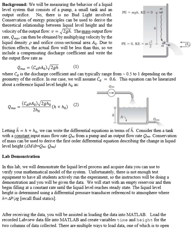
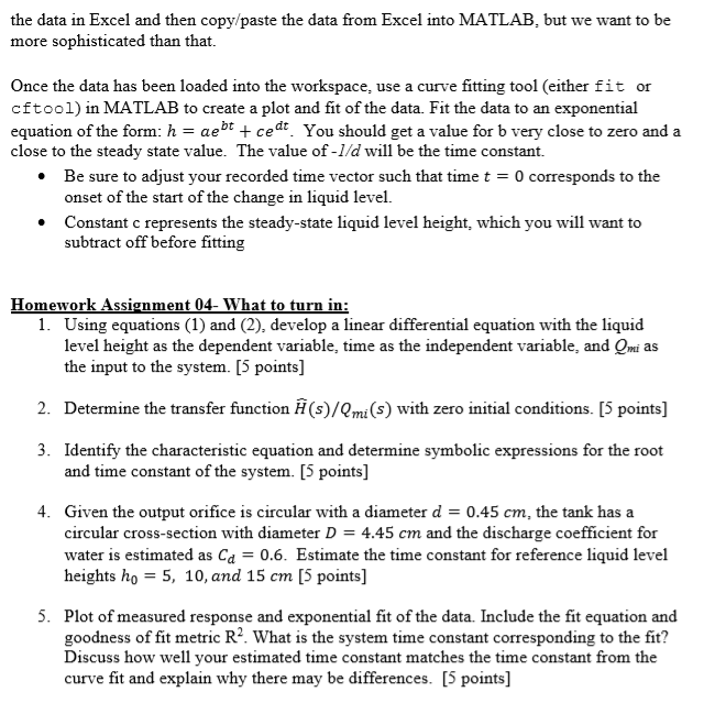
Background: We will be measuring the behavior of a liquid level system that consists of a pump, a small tank and an output orifice. No, there is no Bud Light involved. Conservation of energy principles can be used to derive the theoretical relationship between liquid level height and the velocity of the output flow: v = 2gh. The mass output flow rate, Qmo, can then be obtained by multiplying velocity by the liquid density and orifice cross-sectional area A. Due to friction effects, the actual flow will be less than this, so we include a compensating discharge coefficient and write the the output flow rate as Qmo = (CapAo)2gh (1) PE mgh, KE-0 T PE-0, KE- 2/1 m where Ca is the discharge coefficient and can typically range from 0.5 to 1 depending on the geometry of the orifice. In our case, we will assume Cd = 0.6. This equation can be linearized about a reference liquid level height ho as: Qmi Qmo (CapAo)2gho 2ho (2) (n +ho) Qmo Letting h+ho, we can write the differential equations in terms of . Consider then a tank with a constant input mass flow rate Qmi from a pump and an output flow rate Qmo. Conservation of mass can be used to derive the first order differential equation describing the change in liquid level height (dM/dt=Qmi- Qmo) Lab Demonstration In this lab, we will demonstrate the liquid level process and acquire data you can use to verify your mathematical model of the system. Unfortunately, there is not enough test equipment to have all students actively run the experiment, so the instructors will be doing a demonstration and you will be given the data. We will start with an empty reservoir and then begin filling at a constant rate until the liquid level reaches steady state. The liquid level height is determined using a differential pressure transducer referenced to atmosphere where h=AP/pg [recall fluid statics]. After receiving the data, you will be assisted in loading the data into MATLAB. Load the recorded Labview data file into MATLAB and create variables time and height for the two columns of data collected. There are multiple ways to load data, one of which is to open the data in Excel and then copy/paste the data from Excel into MATLAB, but we want to be more sophisticated than that. Once the data has been loaded into the workspace, use a curve fitting tool (either fit or cftool) in MATLAB to create a plot and fit of the data. Fit the data to an exponential equation of the form: h = aebt + cedt. You should get a value for b very close to zero and a close to the steady state value. The value of -1/d will be the time constant. Be sure to adjust your recorded time vector such that time t = 0 corresponds to the onset of the start of the change in liquid level. Constant c represents the steady-state liquid level height, which you will want to subtract off before fitting Homework Assignment 04- What to turn in: 1. Using equations (1) and (2), develop a linear differential equation with the liquid level height as the dependent variable, time as the independent variable, and Qmi as the input to the system. [5 points] 2. Determine the transfer function (s)/Qmi (5) with zero initial conditions. [5 points] 3. Identify the characteristic equation and determine symbolic expressions for the root and time constant of the system. [5 points] 4. Given the output orifice is circular with a diameter d = 0.45 cm, the tank has a circular cross-section with diameter D = 4.45 cm and the discharge coefficient for water is estimated as C = 0.6. Estimate the time constant for reference liquid level heights ho 5, 10, and 15 cm [5 points] 5. Plot of measured response and exponential fit of the data. Include the fit equation and goodness of fit metric R. What is the system time constant corresponding to the fit? Discuss how well your estimated time constant matches the time constant from the curve fit and explain why there may be differences. [5 points]