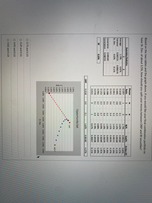
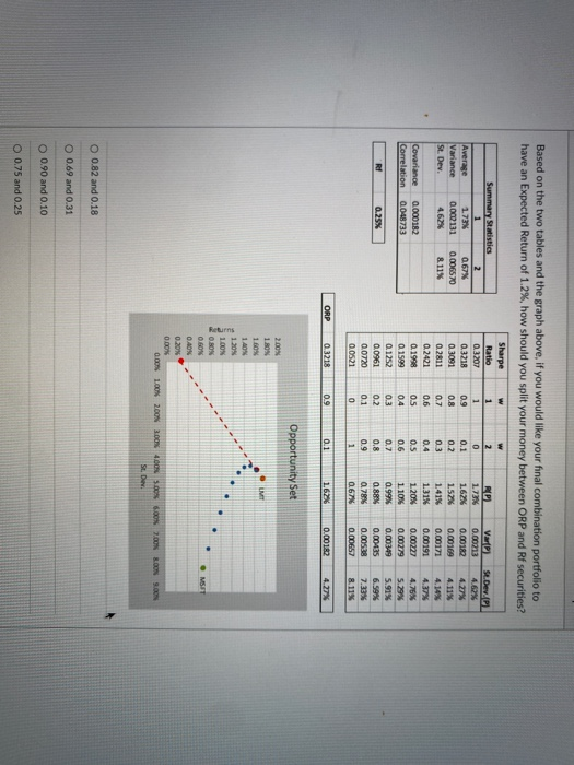
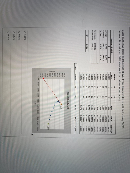
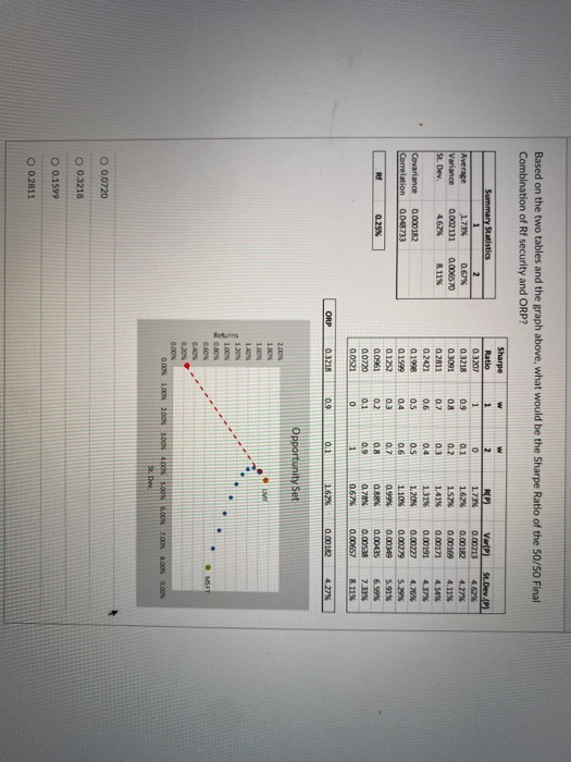
Based on the two tables and the graph above, if you would like your final combination portfolio to have St. Dev. of about 3.5%, how should you split your money between ORP and Rf securities? NE Steve Summary Statistics 2 Average 1.73% 0.67% Variance 0.002131 0.006570 St. Dev. 462 8.11% Sharpe Ratio 0.3207 0.3218 0.3091 0.2811 0.2421 0.1998 0.1599 0.1252 0.0961 0.0720 0.0521 w 1 1 0.9 0.8 0.7 0.6 0.5 0.4 0.3 0.2 0.1 0 2 0 0.1 0.2 03 0.4 0.5 0.6 0.7 08 09 Covariance Correlation RP 17 162% 152 1415 1.31% 1.20% 1.1074 0.99% 0,88% 0.78% 0.67% 4,11% 4.14% 4.37% 0.000182 0008733 Var 0.00213 0.00182 0.00169 0.00171 0.00191 0.00227 0.00279 0.0019 0.00435 0.00578 0.00657 Rf 0.25% 5.29% 5.91% 6.99% 7.33% 8.11% 1 ORP 0.3218 09 0.1 1.62% 0.00182 4.27% Returns Opportunity Set 200N 1.30 1 60W 14N 10 100N O.RO 0.BON MEST QAN 0.200 0.00N 0.00% 1.00% 200N 300N 4.00 . NON BOONOON SL Dev O 0.75 and 0.25 O 0.69 and 0.31 O 0.90 and 0.10 O 0.82 and 0.18 Based on the two tables and the graph above, if you would like your final combination portfolio to have an Expected Return of 1.2%, how should you split your money between ORP and Rf securities? w w 2 St.Dev. 4.62% Average Variance st. Dev. Summary Statistics 2 173N 0.67% 0.002131 0.006570 4.62% 8.11% RP 1.73% 1.62% 1.57% 141 Sharpe Ratio 0.3207 0.3718 0.3091 0.2811 0.2421 0.1998 0.1599 0.1252 0.0961 0.0720 0.0521 Covariance Correlation 0.000182 0018733 1 1 0.9 0.8 0.7 0.6 0.5 04 0.3 0.2 0.1 0 0.1 0.2 03 0.4 0.5 0.6 0.7 0.8 0.9 1 1.31% 1 20 1 10% a 99% 0 88% 078% 0.67 Varta 0.00713 0.00182 0.00169 0.00171 0.00191 0.00227 0.00279 0.00349 0.00435 0.00538 0.00657 4.11% 4.14% 4.37% 4.75% 5.29% 5.91% 6.59% 7.33% 8.11% RI 0.25% ORP 0.3218 09 0.1 1.62% 0.00182 4.27% Opportunity Set 2.00 1 RON 100N LMT Returns 1.30 100N O. BON O.GON . MIT 0.40N 0.20N 0.00 0.00 1.00% 200N 400.00% 5.00% 2.00% ON 3.0 St. Der O 0.82 and 0.18 O 0.69 and 0.31 O 0.90 and 0.10 0.75 and 0.25 Based on the two tables and the graph above, if your client decides to split their money 50/50 between Rf security and ORP, what would be their expected return? w St.Dev. Summary Statistics 2 Average 0.67% Variance 0.002131 0.006570 St. Dev. 4.62% 175 Sharpe Ratio 03207 03218 03091 0 2811 0.2421 0.1998 0 1999 a 1252 0.0961 0.0720 0.0521 w 1 1 0.9 0.8 0.7 0.6 11% Covariance Correlation 2 0 0.1 0.2 0.3 0.4 0.5 0.6 0.7 0.8 0.9 1 0.000182 0.048733 OS Varpi 0.00213 0.00182 0.00169 0.00171 0.00191 0.00227 0.00279 0.00349 0.00015 0.00538 0.00657 1.7 1.62% 152% 1413 1.31% 1.20% 11055 0.99% 0.88% 0.78% 067 477% 4.11% 4.14% 4.37% 4.76% 5.29 5.91% 6.59% 7.33% 8.11% 04 RE 0.25% 03 02 0.1 0 ORP 0.3218 0.9 0.1 16.2% 0.00182 Opportunity Set 2.00 1.ON 160 1.40 LMT Returns 100% O.BOX O BON 0.40N 0.20 MST 0.00 OON 2.00SOON 4.00% 5.00 6.00 78.00 9.00 St. De O 1.20% O 0.81% O 0.94% O 0.16% Based on the two tables and the graph above, what would be the Sharpe Ratio of the 50/50 Final Combination of Rf security and ORP? w 2 St.Dev.01 Summary Statistics 1 2 Average 173 0.67% Variance 0.002131 0.006570 St. Dev. 4.62% 81% 1 1 0.9 08 0.7 Sharpe Ratio 03202 03218 03091 a 2011 02421 a 1998 0 1999 0.1252 0.0961 0.0720 0.0521 0.6 Covariance Correlation 0.000182 0.048733 RO 1.73% 1.62% 15% 1.41% 1.31% 120% 1.10% 0.99 a. BAN 0.78% 0.67% 0.1 0.2 03 0.4 0.5 0.6 0.7 0.8 0.9 1 0.5 04 0.3 0.7 0.1 0.00213 0.00182 0.0016 0.00171 0.00191 0.00227 0.00279 0.00349 0.00435 0.00538 0.00657 4.27% 4.11% 4.14% 4.37% 4.76% 5.29% 5.91% 6.59% 7 33% 8.115 RY 0.25% 0 ORP 0.3218 0.9 0.1 162% 0.00182 4.27% Opportunity Set 2.00% 1 80% 1.50N 1.A0N 120 100N Returns 0.60N MET 0.40 0.20 0.00 0.00% 100N 2DON LONDON 5.0 6.00 7.00 8.00 9.00 3D O 0.0720 O 0.3218 O 0.1599 O 0.2811 Based on the two tables and the graph above, if you would like your final combination portfolio to have St. Dev. of about 3.5%, how should you split your money between ORP and Rf securities? NE Steve Summary Statistics 2 Average 1.73% 0.67% Variance 0.002131 0.006570 St. Dev. 462 8.11% Sharpe Ratio 0.3207 0.3218 0.3091 0.2811 0.2421 0.1998 0.1599 0.1252 0.0961 0.0720 0.0521 w 1 1 0.9 0.8 0.7 0.6 0.5 0.4 0.3 0.2 0.1 0 2 0 0.1 0.2 03 0.4 0.5 0.6 0.7 08 09 Covariance Correlation RP 17 162% 152 1415 1.31% 1.20% 1.1074 0.99% 0,88% 0.78% 0.67% 4,11% 4.14% 4.37% 0.000182 0008733 Var 0.00213 0.00182 0.00169 0.00171 0.00191 0.00227 0.00279 0.0019 0.00435 0.00578 0.00657 Rf 0.25% 5.29% 5.91% 6.99% 7.33% 8.11% 1 ORP 0.3218 09 0.1 1.62% 0.00182 4.27% Returns Opportunity Set 200N 1.30 1 60W 14N 10 100N O.RO 0.BON MEST QAN 0.200 0.00N 0.00% 1.00% 200N 300N 4.00 . NON BOONOON SL Dev O 0.75 and 0.25 O 0.69 and 0.31 O 0.90 and 0.10 O 0.82 and 0.18 Based on the two tables and the graph above, if you would like your final combination portfolio to have an Expected Return of 1.2%, how should you split your money between ORP and Rf securities? w w 2 St.Dev. 4.62% Average Variance st. Dev. Summary Statistics 2 173N 0.67% 0.002131 0.006570 4.62% 8.11% RP 1.73% 1.62% 1.57% 141 Sharpe Ratio 0.3207 0.3718 0.3091 0.2811 0.2421 0.1998 0.1599 0.1252 0.0961 0.0720 0.0521 Covariance Correlation 0.000182 0018733 1 1 0.9 0.8 0.7 0.6 0.5 04 0.3 0.2 0.1 0 0.1 0.2 03 0.4 0.5 0.6 0.7 0.8 0.9 1 1.31% 1 20 1 10% a 99% 0 88% 078% 0.67 Varta 0.00713 0.00182 0.00169 0.00171 0.00191 0.00227 0.00279 0.00349 0.00435 0.00538 0.00657 4.11% 4.14% 4.37% 4.75% 5.29% 5.91% 6.59% 7.33% 8.11% RI 0.25% ORP 0.3218 09 0.1 1.62% 0.00182 4.27% Opportunity Set 2.00 1 RON 100N LMT Returns 1.30 100N O. BON O.GON . MIT 0.40N 0.20N 0.00 0.00 1.00% 200N 400.00% 5.00% 2.00% ON 3.0 St. Der O 0.82 and 0.18 O 0.69 and 0.31 O 0.90 and 0.10 0.75 and 0.25 Based on the two tables and the graph above, if your client decides to split their money 50/50 between Rf security and ORP, what would be their expected return? w St.Dev. Summary Statistics 2 Average 0.67% Variance 0.002131 0.006570 St. Dev. 4.62% 175 Sharpe Ratio 03207 03218 03091 0 2811 0.2421 0.1998 0 1999 a 1252 0.0961 0.0720 0.0521 w 1 1 0.9 0.8 0.7 0.6 11% Covariance Correlation 2 0 0.1 0.2 0.3 0.4 0.5 0.6 0.7 0.8 0.9 1 0.000182 0.048733 OS Varpi 0.00213 0.00182 0.00169 0.00171 0.00191 0.00227 0.00279 0.00349 0.00015 0.00538 0.00657 1.7 1.62% 152% 1413 1.31% 1.20% 11055 0.99% 0.88% 0.78% 067 477% 4.11% 4.14% 4.37% 4.76% 5.29 5.91% 6.59% 7.33% 8.11% 04 RE 0.25% 03 02 0.1 0 ORP 0.3218 0.9 0.1 16.2% 0.00182 Opportunity Set 2.00 1.ON 160 1.40 LMT Returns 100% O.BOX O BON 0.40N 0.20 MST 0.00 OON 2.00SOON 4.00% 5.00 6.00 78.00 9.00 St. De O 1.20% O 0.81% O 0.94% O 0.16% Based on the two tables and the graph above, what would be the Sharpe Ratio of the 50/50 Final Combination of Rf security and ORP? w 2 St.Dev.01 Summary Statistics 1 2 Average 173 0.67% Variance 0.002131 0.006570 St. Dev. 4.62% 81% 1 1 0.9 08 0.7 Sharpe Ratio 03202 03218 03091 a 2011 02421 a 1998 0 1999 0.1252 0.0961 0.0720 0.0521 0.6 Covariance Correlation 0.000182 0.048733 RO 1.73% 1.62% 15% 1.41% 1.31% 120% 1.10% 0.99 a. BAN 0.78% 0.67% 0.1 0.2 03 0.4 0.5 0.6 0.7 0.8 0.9 1 0.5 04 0.3 0.7 0.1 0.00213 0.00182 0.0016 0.00171 0.00191 0.00227 0.00279 0.00349 0.00435 0.00538 0.00657 4.27% 4.11% 4.14% 4.37% 4.76% 5.29% 5.91% 6.59% 7 33% 8.115 RY 0.25% 0 ORP 0.3218 0.9 0.1 162% 0.00182 4.27% Opportunity Set 2.00% 1 80% 1.50N 1.A0N 120 100N Returns 0.60N MET 0.40 0.20 0.00 0.00% 100N 2DON LONDON 5.0 6.00 7.00 8.00 9.00 3D O 0.0720 O 0.3218 O 0.1599 O 0.2811
