basic cost behaviors: visualization
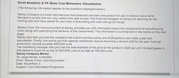
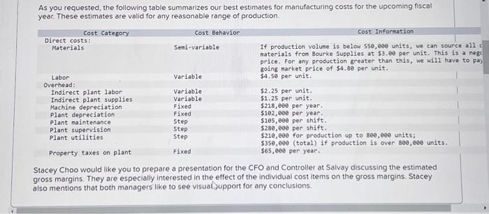
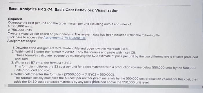
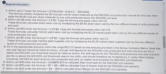
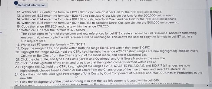
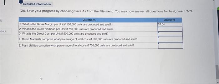
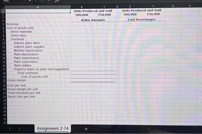
Excel Analytics 2-74: Basic Cost Behaviors: Visualization [The following information applies to the questions displayed below] Salvay Company is a small manufacturer that produces and sells one product for use in medical instruments. Demand is erratic and can vary widely from year to year. The financial managers at Salvay are planning for the coming year and have asked for your help in forecasting unit costs and gross margin. Stacey Choo, the cost accountant at Salvay, provides you with information about the components of manufacturing costs along with specifying the behavior of the components. This information is summarized in the memo on the next page. Stacey also tells you that the company has a zero-inventory policy and all projections are made under that assumption. Finally, she points out that capacity constraints require assuming a second shift for the year if annual production volume exceeds 600,000 units The marketing manager tells you that the best estimate of the price of the product is $20 per unit. His best guess is that demand could be as low as 500,000 units or as high as 750,000 units. Salvay Company Memo: To: Jorge Alcala, Controller From: Stacey Choo, Cost Accountant Date: November 3 . Subject: Cost Information Projections As you requested, the following table summarizes our best estimates for manufacturing costs for the upcoming fiscal year. These estimates are valid for any reasonable range of production. Stacey Choo would like you to prepare a presentation for the CFO and Controller at Salvay discussing the estimated gross margins. They are especially interested in the effect of the individual cost items on the gross margins. Stacey aiso mentions that both managers like to see visual.jupport for any conclusions. Excel Analytics PR 2-74: Basic Cost Behaviors: Visualization Required Compute the cost per unit and the gross margin per unit assuming output and sales of: a. 500,000 units. b. 750,000 units Create a visualization based on your analysis. The relevant data has been included within the following file: Click here to access the Assignment 2-74 Student File. Assignment Steps: 1. Download the Assignment 2-74 Student File and open it within Microsoft Excel 2. Within cell B5 enter the formula =20B2. Copy the formula and paste within cell C5. These formulas calculate revenue by multiplying the $20 estimate of price per unit by the two different levels of units produced and sold. 3. Within cell B7 enter the formula =3B2. This formula multiplies the $3 cost per unit for direct materials with a production volume below 550,000 units by the 500,000 units produced and sold 4. Within cell C7 enter the formula =(3550,000)+(4.8(C2550,000)) This formula initially multiplies the $3 cost per unit for firect materials by the 550,000 unit production volume for this cost, then adds the $4.80 cost per direct materials by any units produced above the 550,000 unit level. 4. Within cell C7 enter the formula =(3550,000)+(4.8(C2550,000)). This formula initially multiplies the $3 cost per unit for direct materials by the 550,000 unit production volume for this cost, then adds the $4.80 cost per direct materials by any units produced above the 550,000 unit level. 5. Within cell 88 enter the formula =4582. Copy the formula and paste within cell C8. These formulas calculate direct labor cost by multiplying the $4.50 direct labor cost by the two different levels of units produced and sold 6. Within cell B10 enter the formula =2.25B2. Copy the formula and paste within cell ClO These formulas calculate indirect plant labor cost by multiplying the $2.25 indirect plant labor cost by the two different levels of units produced and sold. 7. Within cell B11 enter the formula =1.25B2. Copy the formula and paste within cell C11. These formulas calculate indirect plant supplies cost by multiplying the $1.25 indirect plant supplies cost by the two different levels of units produced and sold 8. Fill in the appropriate amounts within the range B12:C17 based on the amounts provided in the Salvay Company Memo. Note that per year figures should be listed as shown, and per shift figures for the 500,000 units produced and sold scenario (as this is below the 600,000 unit threshold) should be listed as shown. Per shift figures for the 750,000 units produced and sold scenario (as this is above the 600,000 unit threshold) require two shifts, and should therefore be multiplied by 2 . Lastly, Plant Utilies should be 210,000 for each level of units produced and sold, as neither level exceeds the 800,000 unit threshold. 9. Within cell B18 enter the formula =SUM(B10:B17) to calsulate Total Overhead for the 500,000 unit scenario, 10. Within cell B19 enter the formula =B7+B8+B18 to calculate Cost of Goods Sold for the 500,000 unit scenario. 11. Within cell 820 enter the formula =85819 to calculate Gross Margin for the 500,000 unit scenario. 12. Within cell 822 enter the formula =819/32 to calculate Cost per Unit for the 500,000 unit scenario. 13. Within cell 823 enter the formula =820/B2 to calculate Gross Margin per Unit for the 500,000 unit scenario. 14. Within cell B24 enter the formula =B18/B2 to calculate Total Overhedd per Unit for the 500,000 unit scenario. 15. Within cell B25 enter the formula =(B7+B8)/B2 to calculate Direct Cost per Unit for the 500,000 unit scenario: 16. Copy the range B18.B25, and paste within the range C18.C25. 17. Within cell E7 enter the formula =87/58519 The dollar signs in front of the column and row references for cell B19 create an absolute cell reference. Absolute formatting ensures that, when copied, a cell reference will be unchanged. This allows the user to copy the formula in cell E7 within a subsequent step. 18. Within cell F7 enter the formula =C7/$C$19 19. Copy the range E7:F7, and paste within both the range E8.F8, and within the range E1O.F17. 20. Highlight the range A2 C2, hold the CTRL key, highlight the range A23.C25 (both ranges are now highlighted), choose Insert Column or Bar Chart from the Charts group of the Insert menu, and select Clustered Bar. 21. Click the chart title, and type Unit Costs (Direct and Overhead) and Unit Gross Margin as the new title 22. Click the background of the chart and drag it so that the top-left corner is located within cell G1. 23. Highlight cell A2, hold the CTRL key, highlight the ranges E2.F2, A7.A8, E7. F8, A10.A17, and E10.F17 (all ranges are now highlighted), choose Insert Column or Bar Chart from the Charts group of the insert menu, and select Clustered Bar. 24. Click the chart title, and type Percentage of Unit Costs by Cost Component at 500,000 and 750,000 Units of Production as the new title. 25. Click the background of the chart and drag it so that the top-left corner is located within cell G16. 26. Save your progress by choosing Save As from the File menu. You may now answer all questions for Assignment 2-74 Excel Analytics 2-74: Basic Cost Behaviors: Visualization [The following information applies to the questions displayed below] Salvay Company is a small manufacturer that produces and sells one product for use in medical instruments. Demand is erratic and can vary widely from year to year. The financial managers at Salvay are planning for the coming year and have asked for your help in forecasting unit costs and gross margin. Stacey Choo, the cost accountant at Salvay, provides you with information about the components of manufacturing costs along with specifying the behavior of the components. This information is summarized in the memo on the next page. Stacey also tells you that the company has a zero-inventory policy and all projections are made under that assumption. Finally, she points out that capacity constraints require assuming a second shift for the year if annual production volume exceeds 600,000 units The marketing manager tells you that the best estimate of the price of the product is $20 per unit. His best guess is that demand could be as low as 500,000 units or as high as 750,000 units. Salvay Company Memo: To: Jorge Alcala, Controller From: Stacey Choo, Cost Accountant Date: November 3 . Subject: Cost Information Projections As you requested, the following table summarizes our best estimates for manufacturing costs for the upcoming fiscal year. These estimates are valid for any reasonable range of production. Stacey Choo would like you to prepare a presentation for the CFO and Controller at Salvay discussing the estimated gross margins. They are especially interested in the effect of the individual cost items on the gross margins. Stacey aiso mentions that both managers like to see visual.jupport for any conclusions. Excel Analytics PR 2-74: Basic Cost Behaviors: Visualization Required Compute the cost per unit and the gross margin per unit assuming output and sales of: a. 500,000 units. b. 750,000 units Create a visualization based on your analysis. The relevant data has been included within the following file: Click here to access the Assignment 2-74 Student File. Assignment Steps: 1. Download the Assignment 2-74 Student File and open it within Microsoft Excel 2. Within cell B5 enter the formula =20B2. Copy the formula and paste within cell C5. These formulas calculate revenue by multiplying the $20 estimate of price per unit by the two different levels of units produced and sold. 3. Within cell B7 enter the formula =3B2. This formula multiplies the $3 cost per unit for direct materials with a production volume below 550,000 units by the 500,000 units produced and sold 4. Within cell C7 enter the formula =(3550,000)+(4.8(C2550,000)) This formula initially multiplies the $3 cost per unit for firect materials by the 550,000 unit production volume for this cost, then adds the $4.80 cost per direct materials by any units produced above the 550,000 unit level. 4. Within cell C7 enter the formula =(3550,000)+(4.8(C2550,000)). This formula initially multiplies the $3 cost per unit for direct materials by the 550,000 unit production volume for this cost, then adds the $4.80 cost per direct materials by any units produced above the 550,000 unit level. 5. Within cell 88 enter the formula =4582. Copy the formula and paste within cell C8. These formulas calculate direct labor cost by multiplying the $4.50 direct labor cost by the two different levels of units produced and sold 6. Within cell B10 enter the formula =2.25B2. Copy the formula and paste within cell ClO These formulas calculate indirect plant labor cost by multiplying the $2.25 indirect plant labor cost by the two different levels of units produced and sold. 7. Within cell B11 enter the formula =1.25B2. Copy the formula and paste within cell C11. These formulas calculate indirect plant supplies cost by multiplying the $1.25 indirect plant supplies cost by the two different levels of units produced and sold 8. Fill in the appropriate amounts within the range B12:C17 based on the amounts provided in the Salvay Company Memo. Note that per year figures should be listed as shown, and per shift figures for the 500,000 units produced and sold scenario (as this is below the 600,000 unit threshold) should be listed as shown. Per shift figures for the 750,000 units produced and sold scenario (as this is above the 600,000 unit threshold) require two shifts, and should therefore be multiplied by 2 . Lastly, Plant Utilies should be 210,000 for each level of units produced and sold, as neither level exceeds the 800,000 unit threshold. 9. Within cell B18 enter the formula =SUM(B10:B17) to calsulate Total Overhead for the 500,000 unit scenario, 10. Within cell B19 enter the formula =B7+B8+B18 to calculate Cost of Goods Sold for the 500,000 unit scenario. 11. Within cell 820 enter the formula =85819 to calculate Gross Margin for the 500,000 unit scenario. 12. Within cell 822 enter the formula =819/32 to calculate Cost per Unit for the 500,000 unit scenario. 13. Within cell 823 enter the formula =820/B2 to calculate Gross Margin per Unit for the 500,000 unit scenario. 14. Within cell B24 enter the formula =B18/B2 to calculate Total Overhedd per Unit for the 500,000 unit scenario. 15. Within cell B25 enter the formula =(B7+B8)/B2 to calculate Direct Cost per Unit for the 500,000 unit scenario: 16. Copy the range B18.B25, and paste within the range C18.C25. 17. Within cell E7 enter the formula =87/58519 The dollar signs in front of the column and row references for cell B19 create an absolute cell reference. Absolute formatting ensures that, when copied, a cell reference will be unchanged. This allows the user to copy the formula in cell E7 within a subsequent step. 18. Within cell F7 enter the formula =C7/$C$19 19. Copy the range E7:F7, and paste within both the range E8.F8, and within the range E1O.F17. 20. Highlight the range A2 C2, hold the CTRL key, highlight the range A23.C25 (both ranges are now highlighted), choose Insert Column or Bar Chart from the Charts group of the Insert menu, and select Clustered Bar. 21. Click the chart title, and type Unit Costs (Direct and Overhead) and Unit Gross Margin as the new title 22. Click the background of the chart and drag it so that the top-left corner is located within cell G1. 23. Highlight cell A2, hold the CTRL key, highlight the ranges E2.F2, A7.A8, E7. F8, A10.A17, and E10.F17 (all ranges are now highlighted), choose Insert Column or Bar Chart from the Charts group of the insert menu, and select Clustered Bar. 24. Click the chart title, and type Percentage of Unit Costs by Cost Component at 500,000 and 750,000 Units of Production as the new title. 25. Click the background of the chart and drag it so that the top-left corner is located within cell G16. 26. Save your progress by choosing Save As from the File menu. You may now answer all questions for Assignment 2-74