Battery Pack $15$ #N$/$A #N$/$A #N$/$A Travel Umbrella B$07$NQKQ$19$S $$11\mathrm{.}08$

Battery Pack $6$ #N$/$A #N$/$A #N$/$A Bluetooth Headphones B$01$NAJGGA$2$ $$33\mathrm{.}02$

Bluetooth Headphones $21$ #N$/$A #N$/$A #N$/$A Battery Pack B$00$Z$9$QVE$4$Q $$34\mathrm{.}88$

Carry$-$on Suitcase $8$ #N$/$A #N$/$A #N$/$A Travel Pillow B$00$GXBZM$5$I $$13\mathrm{.}62$

Travel Umbrella $2$ #N$/$A #N$/$A #N$/$A Carry$-$on Suitcase B$07$PB$3$P$1$N$8$ $$38\mathrm{.}67$

Bluetooth Headphones $4$ #N$/$A #N$/$A #N$/$A

Carry$-$on Suitcase $6$ #N$/$A #N$/$A #N$/$A Pivot Table

Battery Pack $4$ #N$/$A #N$/$A #N$/$A

Battery Pack $15$ #N$/$A #N$/$A #N$/$A

Bluetooth Headphones $24$ #N$/$A #N$/$A #N$/$A

Carry$-$on Suitcase $30$ #N$/$A #N$/$A #N$/$A

Bluetooth Headphones $1$ #N$/$A #N$/$A #N$/$A

Travel Pillow $18$ #N$/$A #N$/$A #N$/$A

Battery Pack $13$ #N$/$A #N$/$A #N$/$A

Travel Umbrella $4$ #N$/$A #N$/$A #N$/$A

Bluetooth Headphones $20$ #N$/$A #N$/$A #N$/$A

Carry$-$on Suitcase $22$ #N$/$A #N$/$A #N$/$A

Bluetooth Headphones $16$ #N$/$A #N$/$A #N$/$A

Travel Umbrella $9$ #N$/$A #N$/$A #N$/$A

Bluetooth Headphones $25$ #N$/$A #N$/$A #N$/$A

Bluetooth Headphones $5$ #N$/$A #N$/$A #N$/$A

Travel Pillow $1$ #N$/$A #N$/$A #N$/$A

Carry$-$on Suitcase $17$ #N$/$A #N$/$A #N$/$A

Travel Pillow $4$ #N$/$A #N$/$A #N$/$A

Bluetooth Headphones $26$ #N$/$A #N$/$A #N$/$A

Travel Pillow $18$ #N$/$A #N$/$A #N$/$A

Travel Pillow $12$ #N$/$A #N$/$A #N$/$A

Travel Pillow $15$ #N$/$A #N$/$A #N$/$A

Travel Pillow $29$ #N$/$A #N$/$A #N$/$A

Travel Umbrella $21$ #N$/$A #N$/$A #N$/$A

Travel Umbrella $4$ #N$/$A #N$/$A #N$/$A

Travel Umbrella $6$ #N$/$A #N$/$A #N$/$A

Carry$-$on Suitcase $25$ #N$/$A #N$/$A #N$/$A

Bluetooth Headphones $24$ #N$/$A #N$/$A #N$/$A

Carry$-$on Suitcase $11$ #N$/$A #N$/$A #N$/$A

Battery Pack $4$ #N$/$A #N$/$A #N$/$A

Carry$-$on Suitcase $7$ #N$/$A #N$/$A #N$/$A

Carry$-$on Suitcase $8$ #N$/$A #N$/$A #N$/$A

Battery Pack $11$ #N$/$A #N$/$A #N$/$A

Bluetooth Headphones $6$ #N$/$A #N$/$A #N$/$A

Travel Pillow $8$ #N$/$A #N$/$A #N$/$A

Carry$-$on Suitcase $9$ #N$/$A #N$/$A #N$/$A

Travel Umbrella $24$ #N$/$A #N$/$A #N$/$A

Carry$-$on Suitcase $4$ #N$/$A #N$/$A #N$/$A

Carry$-$on Suitcase $22$ #N$/$A #N$/$A #N$/$A

Battery Pack $23$ #N$/$A #N$/$A #N$/$A

Bluetooth Headphones $19$ #N$/$A #N$/$A #N$/$A

Bluetooth Headphones $11$ #N$/$A #N$/$A #N$/$A

Carry$-$on Suitcase $5$ #N$/$A #N$/$A #N$/$A

Carry$-$on Suitcase $13$ #N$/$A #N$/$A #N$/$Amath formula, and Excel's fill down feature.

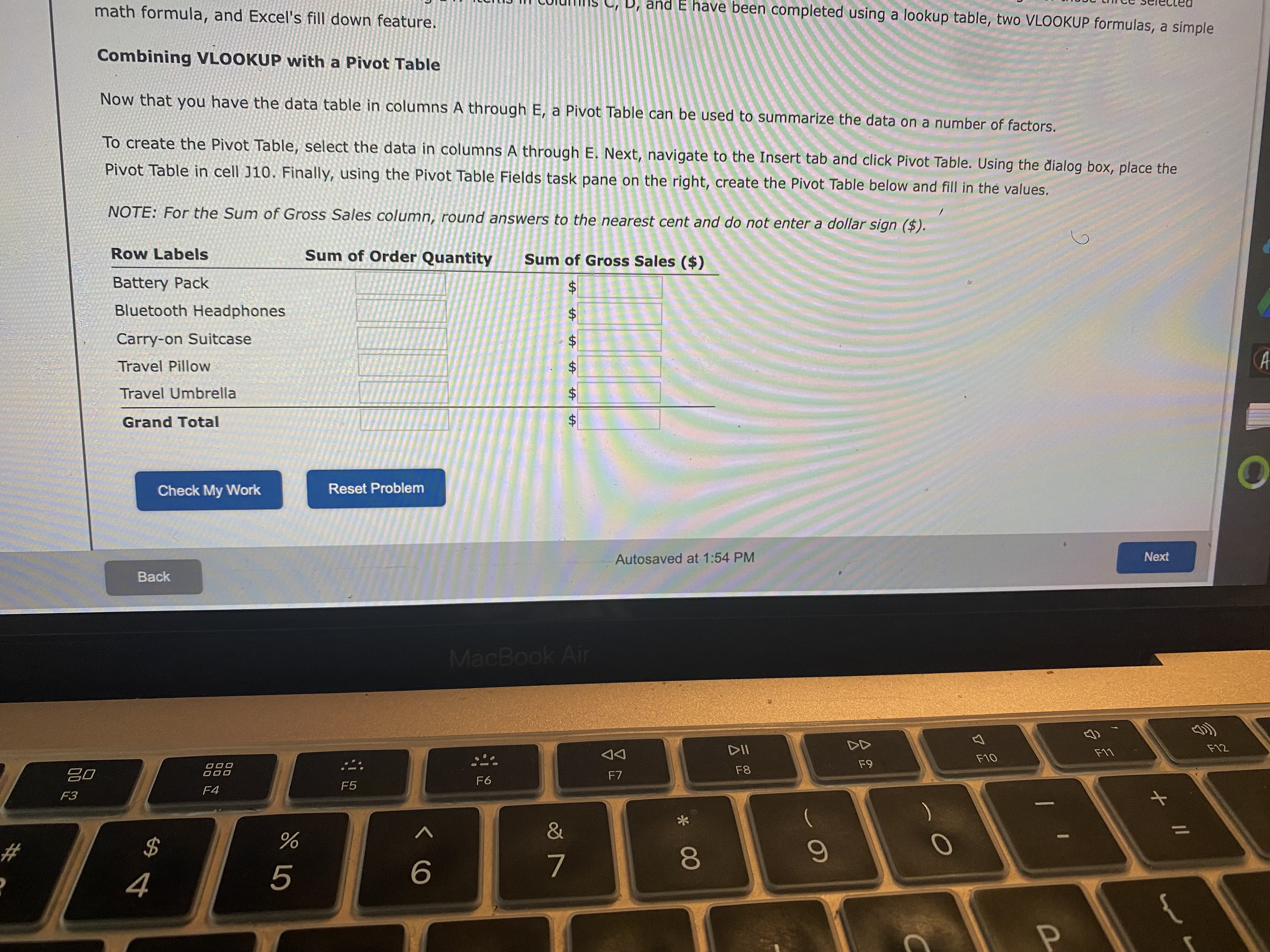
Combining VLOOKUP with a Pivot Table

Now that you have the data table in columns A through E$,$ a Pivot Table can be used to summarize the data on a number of factors.

To create the Pivot Table, select the data in columns A through E$.$ Next, navigate to the Insert tab and click Pivot Table. Using the dialog box, place the

Pivot Table in cell J$10.$ Finally, using the Pivot Table Fields task pane on the right, create the Pivot Table below and fill in the values.

NOTE: For the Sum of Gross Sales column, round answers to the nearest cent and do not enter a dollar sign $($$$).$