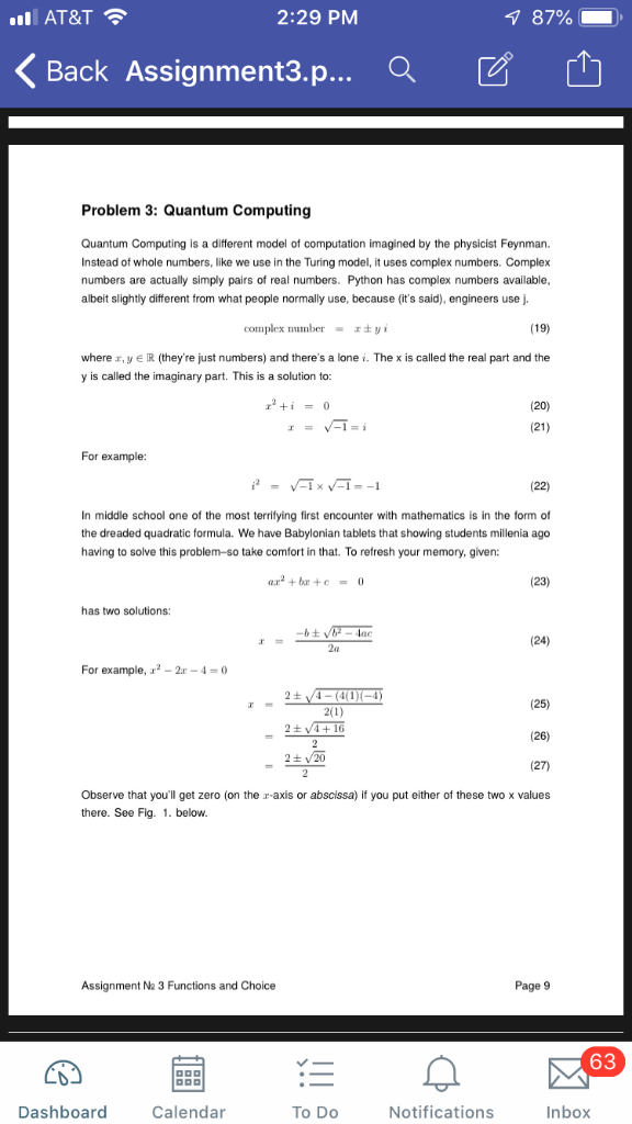
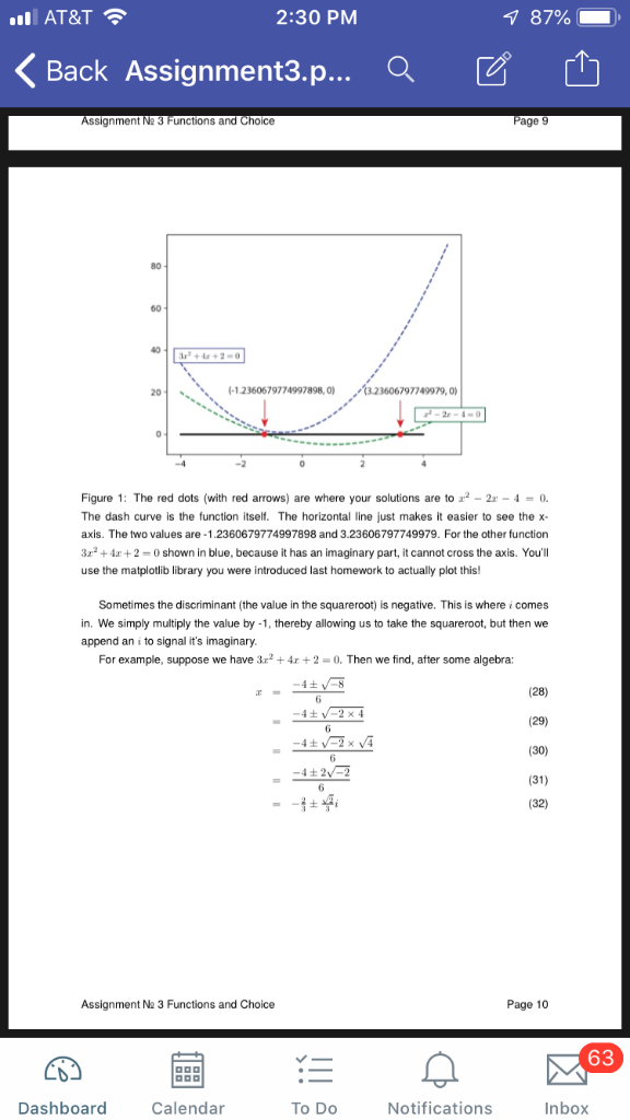
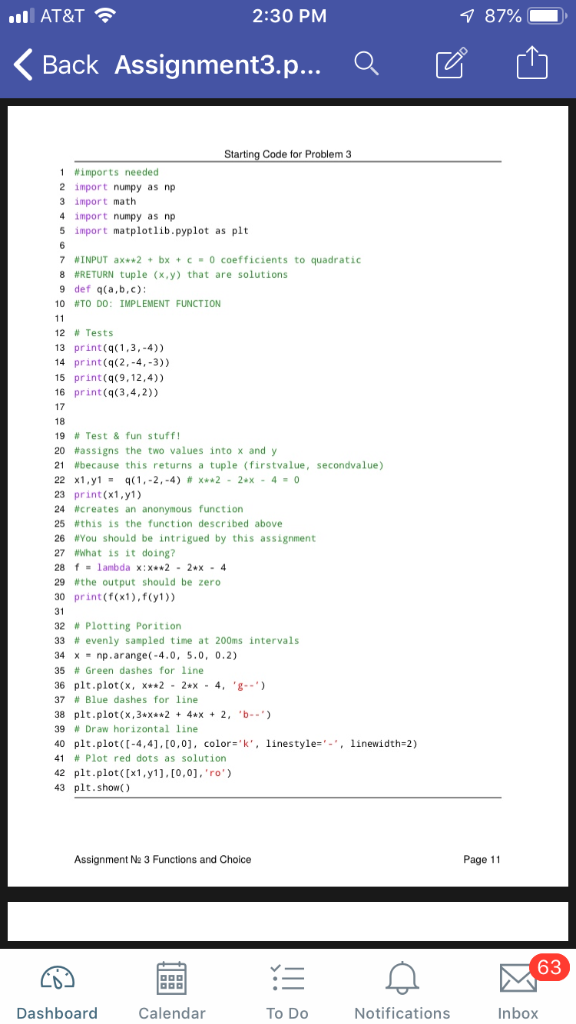
Below are the pictures of each page of the assignment that is given. The goal is to finish the function q that, when tested gives the output shown in the last picture. The code shown in the picture is below:
#imports needed import numpy as np import math import numpy as np import matplotlib.pyplot as plt import cmath
#input ax**2 + bx + c = 0 coefficients to quadratic #RETURN tuple(x,y) that are solutions def q(a,b,c): #TODO: IMPLEMENT FUNCTION #d = (b**2) - (4*a*c) #x = (-b-cmath.sqrt(d))/(2*a) #y = (-b-cmath.sqrt(d))/(2*a)
#Tests print(q(1,3,-4)) print(q(2,-4,-3)) print(q(9,12,4)) print(q(3,4,2))
#Test & fun stuff! #assigns the two values into x and yield #because this returns a tuple (firstvalue, secondvalue) x1,y1 = q(1,-2,-4) #x**2 - 2*x - 4 = 0 print(x1,y1) #creates an anonymous function #this is the function described above #You should be intrigued by this assignment #what is it doing? f = lambda x:x**2 - 2*x - 4 #the output should be zero print(f(x1),f(y1))
#Plotting Porition #evenly sampled time at 200ms intervals x = np.arange(-4.0, 5.0, 0.2) #Green dashes for line plt.plot(x, x**2 - 2*x - 4, 'g--') #Blue dashes for line plt.plot(x, 3*x**2 + 4*x + 2 'b--') #Draw horizontal line plt.plot(-4,4],[0,0], color = 'k', linestyle = '-', linewidth = 2) #Plot red dots as solutions plt.plot([x1,y1],[0,0],'ro') plt.show()


AT&T 2:29 PM 87% Back Assignment3.p Problem 3: Quantum Computing Quantum Computing is a different model of computation imagined by the physicist Feynman. Instead of whole numbers, like we use in the Turing model, it uses complex numbers. Complex numbers are actually simply pairs of real numbers. Python has complex numbers available albeit slightly different from what people normally use, because (it's said), engineers use j. complex number atyi (19) where "r, y e R (they're just numbers) and there's a lone i. The x is called the real part and the y is called the imaginary part. This is a solution to: (20) (21) For example: (22) In middle school one of the most terrifying first encounter with mathematics is in the form of the dreaded quadratic formula. We have Babylonian tablets that showing students millenia ago having to solve this problem-so take comfort in that. To refresh your memory, given: (23) has two solutions: (24) 24 For example, r2-2z-4=0 2 (25) (26) (27) Observe that you'll get zero (on the r-axis or abscissa) if you put either of these two x values 24+16 2t20 there. See Fig. 1. below. Assignment N2 3 Functions and Choice Page 9 63 Dashboard Calendar To Do Notifications Inbox AT&T 2:30 PM Back Assignment3.p Q Assignment N2 3 Functions and Choice Page 9 80 60 r +4+20 20 1.2360679774997898,0) 23606797749979, 0 Figure 1: The red dots (with red arrows) are where your solutions are to 2-2 -4 0 The dash curve is the function itself. The horizontal line just makes it easier to see the x axis. The two values are -1.2360679774997898 and 3.23606797749979. For the other function 3r2 +4+2 0 shown in blue, because it has an imaginary part, it cannot cross the axis. You'll use the matplotlib library you were introduced last homework to actually plot this Sometimes the discriminant (the value in the squareroot) is negative. This is wherei comes in. We simply multiply the value by -1, thereby allowing us to take the squareroot, but then we append an i to signal it's imaginary. For example, suppose we have 3r2 42 0. Then we find, after some algebra: (28) (29) (30) (31) (32) 4+2x4 Assignment Na 3 Functions and Choice Page 10 63 Dashboard Calendar To Do Notifications Inbox AT&T 2:30 PM 87% Back Assignment3.p Q Z Starting Code for Problem 3 I #imports needed 2 import numpy as np 3 import math 4 import numpy as np 5 import matplotlib.pyplot as plt 7 #INPUT ax*+2 + bx + c . 0 coefficients to quadratic 8 #RETURN tuple (x,y) that are solutions 9 def q(a,b,c) 10 #TODO: IMPLEMENT FUNCTION 12 # Tests 13 print(qc1,3,-4)) 14 print (q(2,-4,-3)) 15 print(qc9,12,4)) 16 print (q(3,4,2)) 17 18 19 # Test & fun stuff! 20 #assigns the two values into x and y 21 #because this returns a tuple (firstvalue, secondvalue) 23 print(x1,y1) 24 #creates an anonymous function 25 #this is the function described above 26 WYou should be intrigued by this assignment 27 Wwhat is it doing? 28 1ambda x:x*2 - 2x- 4 29 #the output should be zero 30 print (f(x1), f(y1)) 32 # Plotting Por ition 33 # evenly sampled time at 200ms intervals 34 x = np . arange(-4.0, 5.0, 0.2) 35 # Green dashes for line 36 plt.plot(x, x**2 2x - 4, 'g- 37 # Blue dashes for line 38 plt.plot(x,3x*24*x 2, 'b--) 39 # Draw horizontal line 40 plt.plot(-4,4], [0,0], color linestyle-,linewidth-2) 41 # Plot red dots as solution 42 plt.plot([x1,y1], [0,0], 'ro') 43 plt.showC) Assignment Na 3 Functions and Choice Page 11 63 Dashboard Calendar To Do Notifications Inbox AT&T 2:30 PM Back Assignment3.p Q Output for Problem 3 Not Complex Not Complex (-0.5811388300841898, 2.58113883008419) Not Complex (-0.6666666666666666, -0.6666666666666666) Complex (-0.67+0.47), -0.67-0.47j)) Not Complex 1.2360679774997898 3.23606797749979 0.0 0.0 Assignment N2 3 Functions and Choice Page 12 63 Dashboard Calendar To Do Notifications Inbox AT&T 2:29 PM 87% Back Assignment3.p Problem 3: Quantum Computing Quantum Computing is a different model of computation imagined by the physicist Feynman. Instead of whole numbers, like we use in the Turing model, it uses complex numbers. Complex numbers are actually simply pairs of real numbers. Python has complex numbers available albeit slightly different from what people normally use, because (it's said), engineers use j. complex number atyi (19) where "r, y e R (they're just numbers) and there's a lone i. The x is called the real part and the y is called the imaginary part. This is a solution to: (20) (21) For example: (22) In middle school one of the most terrifying first encounter with mathematics is in the form of the dreaded quadratic formula. We have Babylonian tablets that showing students millenia ago having to solve this problem-so take comfort in that. To refresh your memory, given: (23) has two solutions: (24) 24 For example, r2-2z-4=0 2 (25) (26) (27) Observe that you'll get zero (on the r-axis or abscissa) if you put either of these two x values 24+16 2t20 there. See Fig. 1. below. Assignment N2 3 Functions and Choice Page 9 63 Dashboard Calendar To Do Notifications Inbox AT&T 2:30 PM Back Assignment3.p Q Assignment N2 3 Functions and Choice Page 9 80 60 r +4+20 20 1.2360679774997898,0) 23606797749979, 0 Figure 1: The red dots (with red arrows) are where your solutions are to 2-2 -4 0 The dash curve is the function itself. The horizontal line just makes it easier to see the x axis. The two values are -1.2360679774997898 and 3.23606797749979. For the other function 3r2 +4+2 0 shown in blue, because it has an imaginary part, it cannot cross the axis. You'll use the matplotlib library you were introduced last homework to actually plot this Sometimes the discriminant (the value in the squareroot) is negative. This is wherei comes in. We simply multiply the value by -1, thereby allowing us to take the squareroot, but then we append an i to signal it's imaginary. For example, suppose we have 3r2 42 0. Then we find, after some algebra: (28) (29) (30) (31) (32) 4+2x4 Assignment Na 3 Functions and Choice Page 10 63 Dashboard Calendar To Do Notifications Inbox AT&T 2:30 PM 87% Back Assignment3.p Q Z Starting Code for Problem 3 I #imports needed 2 import numpy as np 3 import math 4 import numpy as np 5 import matplotlib.pyplot as plt 7 #INPUT ax*+2 + bx + c . 0 coefficients to quadratic 8 #RETURN tuple (x,y) that are solutions 9 def q(a,b,c) 10 #TODO: IMPLEMENT FUNCTION 12 # Tests 13 print(qc1,3,-4)) 14 print (q(2,-4,-3)) 15 print(qc9,12,4)) 16 print (q(3,4,2)) 17 18 19 # Test & fun stuff! 20 #assigns the two values into x and y 21 #because this returns a tuple (firstvalue, secondvalue) 23 print(x1,y1) 24 #creates an anonymous function 25 #this is the function described above 26 WYou should be intrigued by this assignment 27 Wwhat is it doing? 28 1ambda x:x*2 - 2x- 4 29 #the output should be zero 30 print (f(x1), f(y1)) 32 # Plotting Por ition 33 # evenly sampled time at 200ms intervals 34 x = np . arange(-4.0, 5.0, 0.2) 35 # Green dashes for line 36 plt.plot(x, x**2 2x - 4, 'g- 37 # Blue dashes for line 38 plt.plot(x,3x*24*x 2, 'b--) 39 # Draw horizontal line 40 plt.plot(-4,4], [0,0], color linestyle-,linewidth-2) 41 # Plot red dots as solution 42 plt.plot([x1,y1], [0,0], 'ro') 43 plt.showC) Assignment Na 3 Functions and Choice Page 11 63 Dashboard Calendar To Do Notifications Inbox AT&T 2:30 PM Back Assignment3.p Q Output for Problem 3 Not Complex Not Complex (-0.5811388300841898, 2.58113883008419) Not Complex (-0.6666666666666666, -0.6666666666666666) Complex (-0.67+0.47), -0.67-0.47j)) Not Complex 1.2360679774997898 3.23606797749979 0.0 0.0 Assignment N2 3 Functions and Choice Page 12 63 Dashboard Calendar To Do Notifications Inbox
