Build an EXCEL model for the Earthlizer problem above such that the model can automatically calculate the projects NPV for any value of the input parameters below (within the range specified below). All other relevant information remains unchanged.
CSM, Inc., is considering a 5-year investment in Earthilizer, a new wholly organic fertilizer made from dairy farm waste. This fertilizer was developed by CSMs ag-division over the past 3 years in response to growing demand from organic farmers for a cheaper alternative and due to increased restrictions on the disposal of cattle manure. The product has undergone extensive testing and satisfies all the regulatory parameters.
If the top management team at the corporate office gives the final go ahead, the project will be up and running by the end of 2019 (end of this year), with first year of sales in 2020. It will require an initial investment in property, plant and equipment (PPE) of $330K (in 2019). The assets have a 10-year life and will be depreciated to zero salvage value over that time on a straight-line basis. The company expects that it can sell the assets at its book value when the project ends at year-end of 2024.
In the first year (2020), sales are expected to be $1 million. Further, they initially assume a conservative project sales growth rate of 0% throughout the 5-year period (till 2024). The COGS is expected to 67.40% of sales and Operating expenses except for depreciation are expected to be 10% of sales (variable expenses) plus an annual fixed expense of $115K.
The projects operating working capital requirement at the end of each year will depend on the project sales of next year. Inventory and Cash requirements will be 20% & 5% of project sales respectively while Accounts Receivables and Account payable will be each be 10% of project sales. Finally, the company estimates that the project will have tax rate of 30%, will be funded entirely with equity capital, and have a cost of capital of 13.25%.


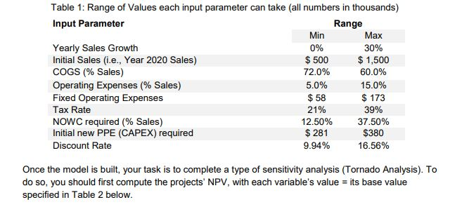
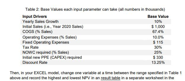
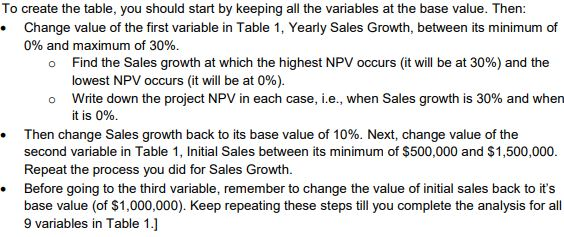
Table 1: Range of Values each input parameter can take (all numbers in thousands) Input Parameter Range Min Max Yearly Sales Growth 0% 30% Initial Sales (i.e., Year 2020 Sales) $ 500 $1,500 COGS (% Sales) 72.0% 60.0% Operating Expenses (% Sales) 5.0% 15.0% Fixed Operating Expenses $ 58 $ 173 Tax Rate 21% 39% NOWC required (% Sales) 12.50% 37.50% Initial new PPE (CAPEX) required $ 281 $380 Discount Rate 9.94% 16.56% Once the model is built, your task is to complete a type of sensitivity analysis (Tornado Analysis). To do so, you should first compute the projects' NPV, with each variable's value = its base value specified in Table 2 below. Table 2: Base Values each input parameter can take all numbers in thousands) Input Drivers Base Value Yearly Sales Growth 10% Initial Sales (i.e., Year 2020 Sales) $ 1,000 COGS (% Sales) 67.4% Operating Expenses (% Sales) 10.0% Fixed Operating Expenses $ 115 Tax Rate 30% NOWC required (% Sales) 25% Initial new PPE (CAPEX) required $ 330 Discount Rate 13.25% Then, in your EXCEL model, change one variable at a time between the range specified in Table 1 above and record the highest and lowest NPV in an result table in a separate worksheet in the o To create the table, you should start by keeping all the variables at the base value. Then: Change value of the first variable in Table 1, Yearly Sales Growth, between its minimum of 0% and maximum of 30%. Find the Sales growth at which the highest NPV occurs (it will be at 30%) and the lowest NPV occurs (it will be at 0%). o Write down the project NPV in each case, i.e., when Sales growth is 30% and when it is 0%. Then change Sales growth back to its base value of 10%. Next, change value of the second variable in Table 1, Initial Sales between its minimum of $500,000 and $1,500,000. Repeat the process you did for Sales Growth. Before going to the third variable, remember to change the value of initial sales back to it's base value of $1,000,000). Keep repeating these steps till you complete the analysis for all 9 variables in Table 1.1 Table 1: Range of Values each input parameter can take (all numbers in thousands) Input Parameter Range Min Max Yearly Sales Growth 0% 30% Initial Sales (i.e., Year 2020 Sales) $ 500 $1,500 COGS (% Sales) 72.0% 60.0% Operating Expenses (% Sales) 5.0% 15.0% Fixed Operating Expenses $ 58 $ 173 Tax Rate 21% 39% NOWC required (% Sales) 12.50% 37.50% Initial new PPE (CAPEX) required $ 281 $380 Discount Rate 9.94% 16.56% Once the model is built, your task is to complete a type of sensitivity analysis (Tornado Analysis). To do so, you should first compute the projects' NPV, with each variable's value = its base value specified in Table 2 below. Table 2: Base Values each input parameter can take all numbers in thousands) Input Drivers Base Value Yearly Sales Growth 10% Initial Sales (i.e., Year 2020 Sales) $ 1,000 COGS (% Sales) 67.4% Operating Expenses (% Sales) 10.0% Fixed Operating Expenses $ 115 Tax Rate 30% NOWC required (% Sales) 25% Initial new PPE (CAPEX) required $ 330 Discount Rate 13.25% Then, in your EXCEL model, change one variable at a time between the range specified in Table 1 above and record the highest and lowest NPV in an result table in a separate worksheet in the o To create the table, you should start by keeping all the variables at the base value. Then: Change value of the first variable in Table 1, Yearly Sales Growth, between its minimum of 0% and maximum of 30%. Find the Sales growth at which the highest NPV occurs (it will be at 30%) and the lowest NPV occurs (it will be at 0%). o Write down the project NPV in each case, i.e., when Sales growth is 30% and when it is 0%. Then change Sales growth back to its base value of 10%. Next, change value of the second variable in Table 1, Initial Sales between its minimum of $500,000 and $1,500,000. Repeat the process you did for Sales Growth. Before going to the third variable, remember to change the value of initial sales back to it's base value of $1,000,000). Keep repeating these steps till you complete the analysis for all 9 variables in Table
