can someone help me with this and send to me?

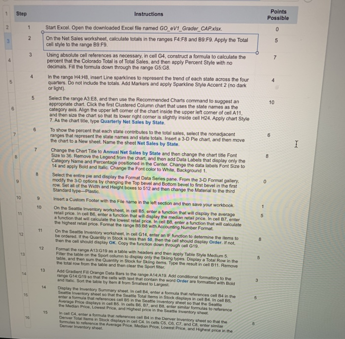
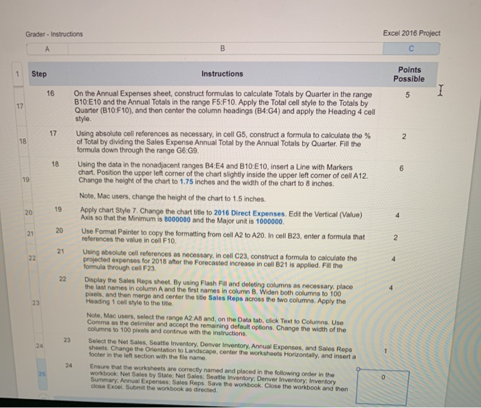
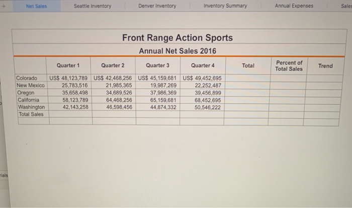
Points Possible Instructions Step Start Excel. Open the downloaded Excel file named GO_eV1_Grader CAP.xisx. 2. 5 On the Net Sales worksheet, calculate totals in the ranges F4:F8 and B9:F9. Apply the Total cell style to the range B9:F9. 3. Using absolute cell references as necessary, in cell G4, construct a formula to calculate the percent that the Colorado Total is of Total Sales, and then apply Percent Style with no decimals. Fill the formula down through the range G5:G8. In the range H4:H8, insert Line sparklines to represent the trend of each state across the four quarters. Do not include the totals. Add Markers and apply Sparkline Style Accent 2 (no dark or light). 4. Select the range A3:E8, and then use the Recommended Charts command to suggest an appropriate chart. Click the first Clustered Column chart that uses the state names as the category axis. Align the upper left comer of the chart inside the upper left corner of cell A11, and then size the chart so that its lower right corner is slightly inside cell H24. Apply chart Style 7. As the chart title, type Quarterly Net Sales by State. 10 To show the percent that each state contributes to the total sales, select the nonadjacent ranges that represent the state names and state totals. Insert a 3-D Pie chart, and then move the chart to a New sheet. Name the sheet Net Sales by State. 6. Change the Chart Title to Annual Net Sales by State and then change the chart title Font Size to 36. Remove the Legend from the chart, and then add Data Labels that display only the Category Name and Percentage positioned in the Center. Change the data labels Font Size to 14 and apply Bold and Italic. Change the Font color to White, Background 1. Select the entire pie and display the Format Data Series pane. From the 3-D Format gallery, modify the 3-D options by changing the Top bevel and Bottom bevel to first bevel in the first row. Set all of the Width and Height boxes to 512 and then change the Material to the third Standard type-Plastic. Insert a Custom Footer with the File name in the left section and then save your workbook 10 On the Seattle Inventory worksheet, in cell B5, enter a function that will display the average retail price. In cell B6, enter a function that will display the median retail price. In cell B7, enter a function that will calculate the lowest retail price. In cell B8, enter a function that will calculate the highest retail price. Format the range B5:B8 with Accounting Number Format. 10 11 On the Seattle Inventory worksheet, in cell G14, enter an IF function to determine the items to be ordered. If the Quantity in Stock is less than 50, then the cell should display Order. If not, then the cell should display OK. Copy the function down through cell G19. 11 12 Format the range A13:G19 as a table with headers and then apply Table Style Medium 5. Filter the table on the Sport column to display only the Skiing types. Display a Total Row in the table, and then sum the Quantity in Stock for Sking items. Type the result in cell B11. Remove the total row from the table and then clear the Sport fiter. 12 13 Add Gradient Fill Orange Data Bars to the range A14:A19. Add conditional formatting to the range G14:G19 so that the cells with text that contain the word Order are formatted with Bold and Italic. Sort the table by Item from Smallest to Largest. 13 14 Display the Inventory Summary sheet In cell B4, enter a formula that references cell B4 in the Seattle Inventory sheet so that the Seattle Total Items in Stock displays in cel B4. In cell B5. enter a formula that references cell B5 in the Seattle Inventory sheet so that the Seattle Average Price displays in cell B5. In cells B6, B7, and B8, enter similar formulas to reference the Median Price, Lowest Price, and Highest price in the Seattle Inventory sheet. 14 15 15 In cell C4, enter a formula that references cell B4 in the Denver Inventory sheet so that the Denver Total Items in Stock displays in cell C4. In cells C5, C6, C7, and C8, enter similar formulas to reference the Average Price. Median Price, Lowest Price, and Highest price in the Denver Inventory sheet 16 Excel 2016 Project Grader - Instructions Points Possible Step Instructions 16 On the Annual Expenses sheet, construct formulas to calculate Totals by Quarter in the range B10:E10 and the Annual Totals in the range F5:F10. Apply the Total cell style to the Totals by Quarter (B10:F10), and then center the column headings (B4:G4) and apply the Heading 4 cell style. 17 Using absolute cell references as necessary, in cell G5, construct a formula to calculate the % of Total by dividing the Sales Expense Annual Total by the Annual Totals by Quarter. Fill the formula down through the range G6:G9. 17 18 Using the data in the nonadjacent ranges B4:E4 and B10:E10, insert a Line with Markers chart. Position the upper left corner of the chart slightly inside the upper left corner of cell A12. Change the height of the chart to 1.75 inches and the width of the chart to 8 inches. 18 19 Note, Mac users, change the height of the chart to 1.5 inches. 19 Apply chart Style 7. Change the chart title to 2016 Direct Expenses. Edit the Vertical (Value) Axis so that the Minimum is 8000000 and the Major unit is 1000000. 20 20 Use Format Painter to copy the formatting from cell A2 to A20. In cell B23, enter a formula that references the value in cell F10. 21 2 21 Using absolute cell references as necessary, in cell C23, construct a formula to calculate the projected expenses for 2018 after the Forecasted increase in cell B21 is applied. Fill the formula through cell F23. 22 22 Display the Sales Reps sheet. By using Flash Fill and deleting columns as necessary, place the last names in column A and the first names in column B. Widen both columns to 100 pixels, and then merge and center the title Sales Reps across the two columns. Apply the Heading 1 cell style to the title. 23 Note, Mac users, select the range A2 A8 and, on the Data tab, click Text to Columns. Use Comma as the delimiter and accept the remaining default options. Change the width of the columns to 100 pixels and continue with the instructions. 23 Select the Net Sales, Seattle Inventory, Denver Inventory, Annual Expenses, and Sales Reps sheets. Change the Orientation to Landscape, center the worksheets Horizontally, and insert a footer in the left section with the file name. 24 24 Ensure that the worksheets are correctly named and placed in the following order in the workbook: Net Sales by State: Net Sales: Seatle Inventory: Denver Inventory, Inventory Summary, Annual Expenses: Sales Reps. Save the workbook. Close the workbook and then close Excel. Submit the workbook as directed. 25 Annual Expenses Seattle Inventory Denver Inventory Inventory Summary Sales Net Sales Front Range Action Sports Annual Net Sales 2016 Percent of Quarter 3 Total Quarter 1 Quarter 2 Quarter 4 Trend Total Sales Colorado New Mexico Oregon California Washington US$ 48,123,789 US$ 42,468,256 US$ 45,159,681 19,987,269 37,986,369 USS 49,452,695 21,985,365 25,783,516 22,252,487 35,658,498 34,689,526 39,456,899 58,123,789 64,468,256 65,159,681 68,452,695 42,143,258 46,598,456 44,874,332 50,546,222 Total Sales rials Points Possible Instructions Step Start Excel. Open the downloaded Excel file named GO_eV1_Grader CAP.xisx. 2. 5 On the Net Sales worksheet, calculate totals in the ranges F4:F8 and B9:F9. Apply the Total cell style to the range B9:F9. 3. Using absolute cell references as necessary, in cell G4, construct a formula to calculate the percent that the Colorado Total is of Total Sales, and then apply Percent Style with no decimals. Fill the formula down through the range G5:G8. In the range H4:H8, insert Line sparklines to represent the trend of each state across the four quarters. Do not include the totals. Add Markers and apply Sparkline Style Accent 2 (no dark or light). 4. Select the range A3:E8, and then use the Recommended Charts command to suggest an appropriate chart. Click the first Clustered Column chart that uses the state names as the category axis. Align the upper left comer of the chart inside the upper left corner of cell A11, and then size the chart so that its lower right corner is slightly inside cell H24. Apply chart Style 7. As the chart title, type Quarterly Net Sales by State. 10 To show the percent that each state contributes to the total sales, select the nonadjacent ranges that represent the state names and state totals. Insert a 3-D Pie chart, and then move the chart to a New sheet. Name the sheet Net Sales by State. 6. Change the Chart Title to Annual Net Sales by State and then change the chart title Font Size to 36. Remove the Legend from the chart, and then add Data Labels that display only the Category Name and Percentage positioned in the Center. Change the data labels Font Size to 14 and apply Bold and Italic. Change the Font color to White, Background 1. Select the entire pie and display the Format Data Series pane. From the 3-D Format gallery, modify the 3-D options by changing the Top bevel and Bottom bevel to first bevel in the first row. Set all of the Width and Height boxes to 512 and then change the Material to the third Standard type-Plastic. Insert a Custom Footer with the File name in the left section and then save your workbook 10 On the Seattle Inventory worksheet, in cell B5, enter a function that will display the average retail price. In cell B6, enter a function that will display the median retail price. In cell B7, enter a function that will calculate the lowest retail price. In cell B8, enter a function that will calculate the highest retail price. Format the range B5:B8 with Accounting Number Format. 10 11 On the Seattle Inventory worksheet, in cell G14, enter an IF function to determine the items to be ordered. If the Quantity in Stock is less than 50, then the cell should display Order. If not, then the cell should display OK. Copy the function down through cell G19. 11 12 Format the range A13:G19 as a table with headers and then apply Table Style Medium 5. Filter the table on the Sport column to display only the Skiing types. Display a Total Row in the table, and then sum the Quantity in Stock for Sking items. Type the result in cell B11. Remove the total row from the table and then clear the Sport fiter. 12 13 Add Gradient Fill Orange Data Bars to the range A14:A19. Add conditional formatting to the range G14:G19 so that the cells with text that contain the word Order are formatted with Bold and Italic. Sort the table by Item from Smallest to Largest. 13 14 Display the Inventory Summary sheet In cell B4, enter a formula that references cell B4 in the Seattle Inventory sheet so that the Seattle Total Items in Stock displays in cel B4. In cell B5. enter a formula that references cell B5 in the Seattle Inventory sheet so that the Seattle Average Price displays in cell B5. In cells B6, B7, and B8, enter similar formulas to reference the Median Price, Lowest Price, and Highest price in the Seattle Inventory sheet. 14 15 15 In cell C4, enter a formula that references cell B4 in the Denver Inventory sheet so that the Denver Total Items in Stock displays in cell C4. In cells C5, C6, C7, and C8, enter similar formulas to reference the Average Price. Median Price, Lowest Price, and Highest price in the Denver Inventory sheet 16 Excel 2016 Project Grader - Instructions Points Possible Step Instructions 16 On the Annual Expenses sheet, construct formulas to calculate Totals by Quarter in the range B10:E10 and the Annual Totals in the range F5:F10. Apply the Total cell style to the Totals by Quarter (B10:F10), and then center the column headings (B4:G4) and apply the Heading 4 cell style. 17 Using absolute cell references as necessary, in cell G5, construct a formula to calculate the % of Total by dividing the Sales Expense Annual Total by the Annual Totals by Quarter. Fill the formula down through the range G6:G9. 17 18 Using the data in the nonadjacent ranges B4:E4 and B10:E10, insert a Line with Markers chart. Position the upper left corner of the chart slightly inside the upper left corner of cell A12. Change the height of the chart to 1.75 inches and the width of the chart to 8 inches. 18 19 Note, Mac users, change the height of the chart to 1.5 inches. 19 Apply chart Style 7. Change the chart title to 2016 Direct Expenses. Edit the Vertical (Value) Axis so that the Minimum is 8000000 and the Major unit is 1000000. 20 20 Use Format Painter to copy the formatting from cell A2 to A20. In cell B23, enter a formula that references the value in cell F10. 21 2 21 Using absolute cell references as necessary, in cell C23, construct a formula to calculate the projected expenses for 2018 after the Forecasted increase in cell B21 is applied. Fill the formula through cell F23. 22 22 Display the Sales Reps sheet. By using Flash Fill and deleting columns as necessary, place the last names in column A and the first names in column B. Widen both columns to 100 pixels, and then merge and center the title Sales Reps across the two columns. Apply the Heading 1 cell style to the title. 23 Note, Mac users, select the range A2 A8 and, on the Data tab, click Text to Columns. Use Comma as the delimiter and accept the remaining default options. Change the width of the columns to 100 pixels and continue with the instructions. 23 Select the Net Sales, Seattle Inventory, Denver Inventory, Annual Expenses, and Sales Reps sheets. Change the Orientation to Landscape, center the worksheets Horizontally, and insert a footer in the left section with the file name. 24 24 Ensure that the worksheets are correctly named and placed in the following order in the workbook: Net Sales by State: Net Sales: Seatle Inventory: Denver Inventory, Inventory Summary, Annual Expenses: Sales Reps. Save the workbook. Close the workbook and then close Excel. Submit the workbook as directed. 25 Annual Expenses Seattle Inventory Denver Inventory Inventory Summary Sales Net Sales Front Range Action Sports Annual Net Sales 2016 Percent of Quarter 3 Total Quarter 1 Quarter 2 Quarter 4 Trend Total Sales Colorado New Mexico Oregon California Washington US$ 48,123,789 US$ 42,468,256 US$ 45,159,681 19,987,269 37,986,369 USS 49,452,695 21,985,365 25,783,516 22,252,487 35,658,498 34,689,526 39,456,899 58,123,789 64,468,256 65,159,681 68,452,695 42,143,258 46,598,456 44,874,332 50,546,222 Total Sales rials
