CAN SOMEONE PLEASE HELP ME WITH THE ENTIRETY OF THIS QUESTION? HELP IS NEEDED PLEASE

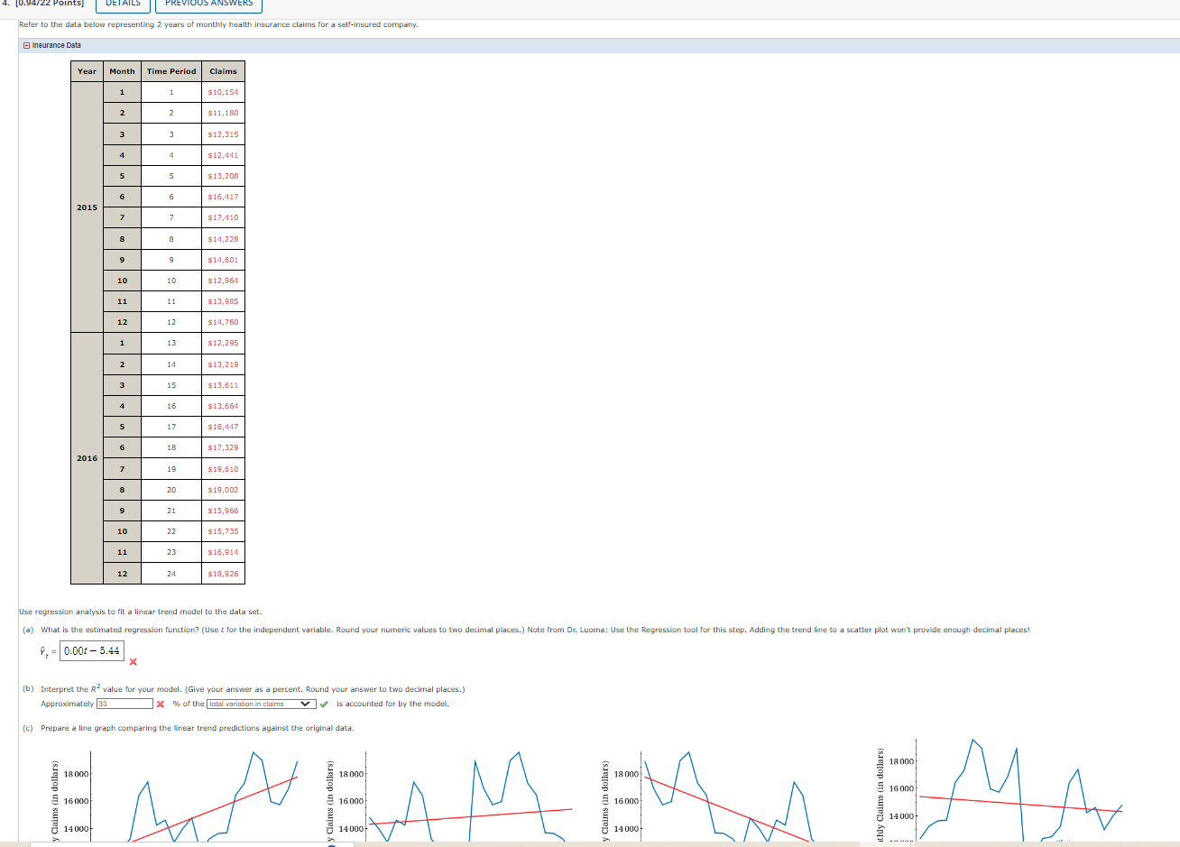
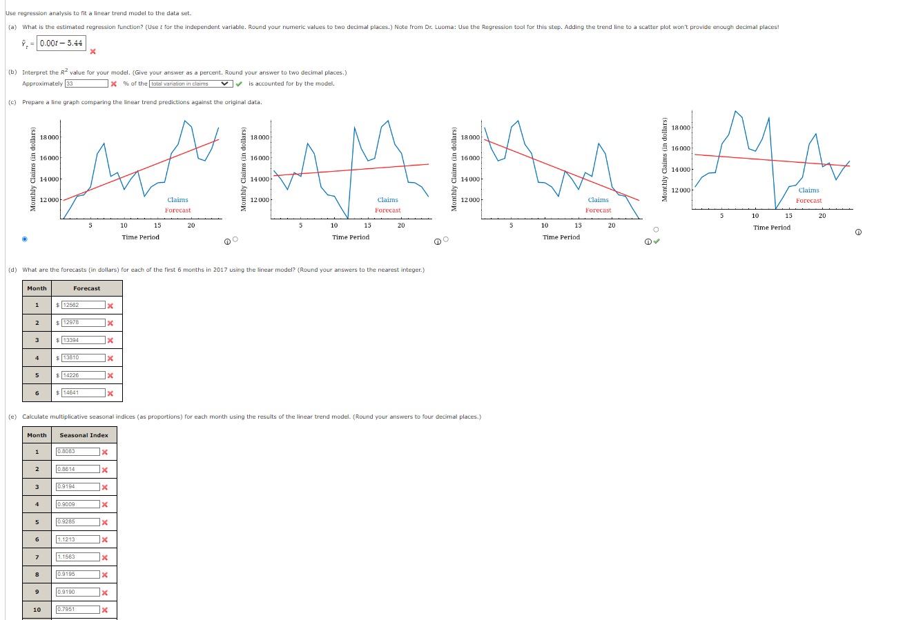
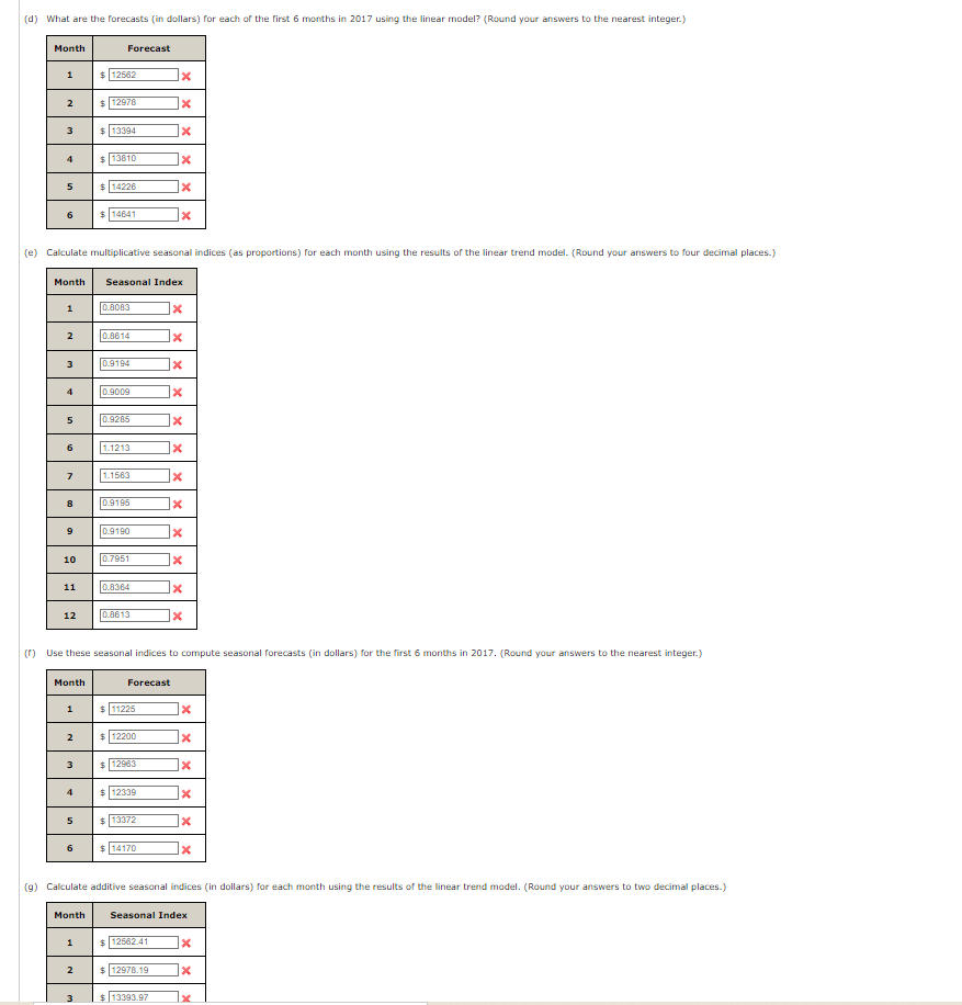
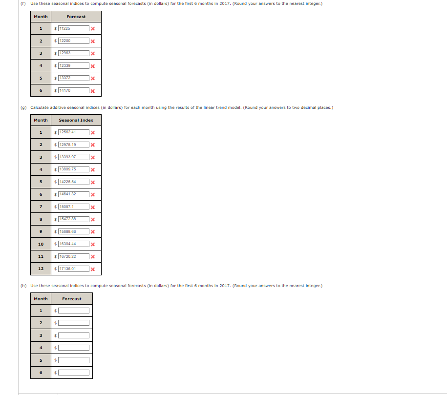
Use regression analysis to fit a linear trend model to the data set. Y^t= x (b) Interpret the R2 value for your model. (Give your answer as a percent. Round your answer to two decimal places.) Approximately % of the total variation in claims is accounted for by the model. (c) Prepare a line graph comparing the linear trend predictions against the original data. Jse regression analysis to fit a linear trend model to the data set. Y^t= x (b) Interpret the R2 value for your model. (Give your answer as a percent. Round your answer to two decimal places.) Approximately of the is accounted for by the model. (c) Prepare a line graph comparing the linear trend predictions against the original data. (d) What are the forecasts (in dollars) for each of the first 6 months in 2017 using the linear model? (Round your answers to the nearest integer.) (d) What are the forecasts (in dollars) for each of the first 6 months in 2017 using the linear model? (Round your answers to the nearest integer.) \begin{tabular}{|c|c|} \hline Month & \multicolumn{2}{|c|}{ Forecast } \\ \hline 1 & $12562 \\ \hline 2 & $12978 \\ \hline 3 & $13394 \\ \hline 4 & $13810 \\ \hline 5 & $14226 \\ \hline 6 & $14841 \\ \hline \end{tabular} (e) Calculate multiplicative seasonal indices (as proportions) for each month using the results of the linear trend model. (Round your answers to four decimal places.) \begin{tabular}{|c|l|} \hline Month & \multicolumn{1}{|c|}{ Seasonal Index } \\ \hline 1 & 0.9083 \\ \hline 2 & 0.9614 \\ \hline 3 & 0.9194 \\ \hline 4 & 0.9009 \\ \hline 5 & 0.9285 \\ \hline 6 & 1.1213 \\ \hline 7 & 1.1563 \\ \hline 8 & 0.9195 \\ \hline 9 & 0.9190 \\ \hline 10 & 0.7951 \\ \hline 11 & 0.8364 \\ \hline 12 & 0.9613 \\ \hline \end{tabular} (f) Use these seasonal indices to compute seasonal forecasts (in dollars) for the first 6 months in 2017. (Round your answers to the nearest integer.) \begin{tabular}{|c|c|} \hline Month & \multicolumn{1}{|c|}{ Forecast } \\ \hline 1 & $11225 \\ \hline 2 & $12200 \\ \hline 3 & $12963 \\ \hline 4 & $12339 \\ \hline 5 & $13372 \\ \hline 6 & $14170 \\ \hline \end{tabular} (9) Calculate additive seasonal indices (in dollars) for each month using the results of the linear trend model. (Round your answers to two decimal places.) \begin{tabular}{|c|c|} \hline Month & Seasonal Index \\ \hline 1 & $12562.41 \\ \hline 2 & $12978.19 \\ \hline 3 & $13393.97 \\ \hline \end{tabular} (f) Use these seasonal indices to compute seasonal forecasts (in dollars) for the first 6 months in 2017. (Round your answers to the nearest integer.) \begin{tabular}{|c|c|} \hline Month & \multicolumn{1}{|c|}{ Forecast } \\ \hline 1 & $11225 \\ \hline 2 & $12200 \\ \hline 3 & $12963 \\ \hline 4 & $12339 \\ \hline 5 & $13372 \\ \hline 6 & $14170 \\ \hline \end{tabular} (9) Calculate additive seasonal indices (in dollars) for each month using the results of the linear trend model. (Round your answers to two decimal places.) \begin{tabular}{|c|c|} \hline Month & \multicolumn{2}{|c|}{ Seasonal Index } \\ \hline 1 & $12562.41 \\ \hline 2 & $12978.19 \\ \hline 3 & $13393.97 \\ \hline 4 & $13809.75 \\ \hline 5 & $14225.54 \\ \hline 6 & $14841.32 \\ \hline 7 & $15057.1 \\ \hline 8 & $15472.86 \\ \hline 9 & $15886.66 \\ \hline 10 & $16304.44 \\ \hline 11 & $16720.22 \\ \hline 12 & $17136.01 \\ \hline \end{tabular} (h) Use these seasonal indices to compute seasonal forecasts (in dollars) for the first 6 months in 2017. (Round your answers to the nearest integer.) \begin{tabular}{|c|c|} \hline Month & Forecast \\ \hline 1 & $ \\ \hline 2 & $ \\ \hline 3 & $ \\ \hline 4 & $ \\ \hline 5 & $ \\ \hline 6 & $ \\ \hline \end{tabular} Use regression analysis to fit a linear trend model to the data set. Y^t= x (b) Interpret the R2 value for your model. (Give your answer as a percent. Round your answer to two decimal places.) Approximately % of the total variation in claims is accounted for by the model. (c) Prepare a line graph comparing the linear trend predictions against the original data. Jse regression analysis to fit a linear trend model to the data set. Y^t= x (b) Interpret the R2 value for your model. (Give your answer as a percent. Round your answer to two decimal places.) Approximately of the is accounted for by the model. (c) Prepare a line graph comparing the linear trend predictions against the original data. (d) What are the forecasts (in dollars) for each of the first 6 months in 2017 using the linear model? (Round your answers to the nearest integer.) (d) What are the forecasts (in dollars) for each of the first 6 months in 2017 using the linear model? (Round your answers to the nearest integer.) \begin{tabular}{|c|c|} \hline Month & \multicolumn{2}{|c|}{ Forecast } \\ \hline 1 & $12562 \\ \hline 2 & $12978 \\ \hline 3 & $13394 \\ \hline 4 & $13810 \\ \hline 5 & $14226 \\ \hline 6 & $14841 \\ \hline \end{tabular} (e) Calculate multiplicative seasonal indices (as proportions) for each month using the results of the linear trend model. (Round your answers to four decimal places.) \begin{tabular}{|c|l|} \hline Month & \multicolumn{1}{|c|}{ Seasonal Index } \\ \hline 1 & 0.9083 \\ \hline 2 & 0.9614 \\ \hline 3 & 0.9194 \\ \hline 4 & 0.9009 \\ \hline 5 & 0.9285 \\ \hline 6 & 1.1213 \\ \hline 7 & 1.1563 \\ \hline 8 & 0.9195 \\ \hline 9 & 0.9190 \\ \hline 10 & 0.7951 \\ \hline 11 & 0.8364 \\ \hline 12 & 0.9613 \\ \hline \end{tabular} (f) Use these seasonal indices to compute seasonal forecasts (in dollars) for the first 6 months in 2017. (Round your answers to the nearest integer.) \begin{tabular}{|c|c|} \hline Month & \multicolumn{1}{|c|}{ Forecast } \\ \hline 1 & $11225 \\ \hline 2 & $12200 \\ \hline 3 & $12963 \\ \hline 4 & $12339 \\ \hline 5 & $13372 \\ \hline 6 & $14170 \\ \hline \end{tabular} (9) Calculate additive seasonal indices (in dollars) for each month using the results of the linear trend model. (Round your answers to two decimal places.) \begin{tabular}{|c|c|} \hline Month & Seasonal Index \\ \hline 1 & $12562.41 \\ \hline 2 & $12978.19 \\ \hline 3 & $13393.97 \\ \hline \end{tabular} (f) Use these seasonal indices to compute seasonal forecasts (in dollars) for the first 6 months in 2017. (Round your answers to the nearest integer.) \begin{tabular}{|c|c|} \hline Month & \multicolumn{1}{|c|}{ Forecast } \\ \hline 1 & $11225 \\ \hline 2 & $12200 \\ \hline 3 & $12963 \\ \hline 4 & $12339 \\ \hline 5 & $13372 \\ \hline 6 & $14170 \\ \hline \end{tabular} (9) Calculate additive seasonal indices (in dollars) for each month using the results of the linear trend model. (Round your answers to two decimal places.) \begin{tabular}{|c|c|} \hline Month & \multicolumn{2}{|c|}{ Seasonal Index } \\ \hline 1 & $12562.41 \\ \hline 2 & $12978.19 \\ \hline 3 & $13393.97 \\ \hline 4 & $13809.75 \\ \hline 5 & $14225.54 \\ \hline 6 & $14841.32 \\ \hline 7 & $15057.1 \\ \hline 8 & $15472.86 \\ \hline 9 & $15886.66 \\ \hline 10 & $16304.44 \\ \hline 11 & $16720.22 \\ \hline 12 & $17136.01 \\ \hline \end{tabular} (h) Use these seasonal indices to compute seasonal forecasts (in dollars) for the first 6 months in 2017. (Round your answers to the nearest integer.) \begin{tabular}{|c|c|} \hline Month & Forecast \\ \hline 1 & $ \\ \hline 2 & $ \\ \hline 3 & $ \\ \hline 4 & $ \\ \hline 5 & $ \\ \hline 6 & $ \\ \hline \end{tabular}