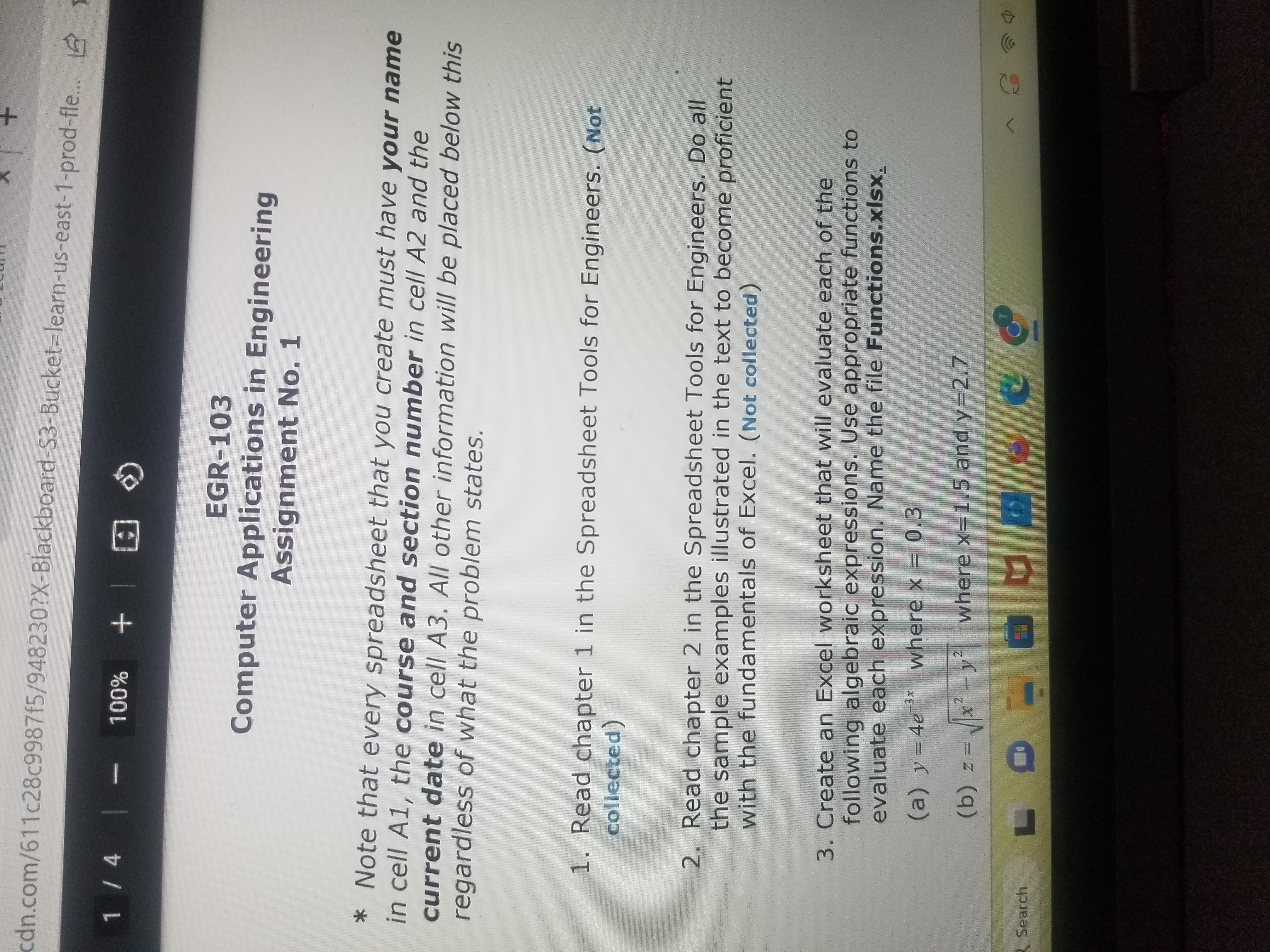
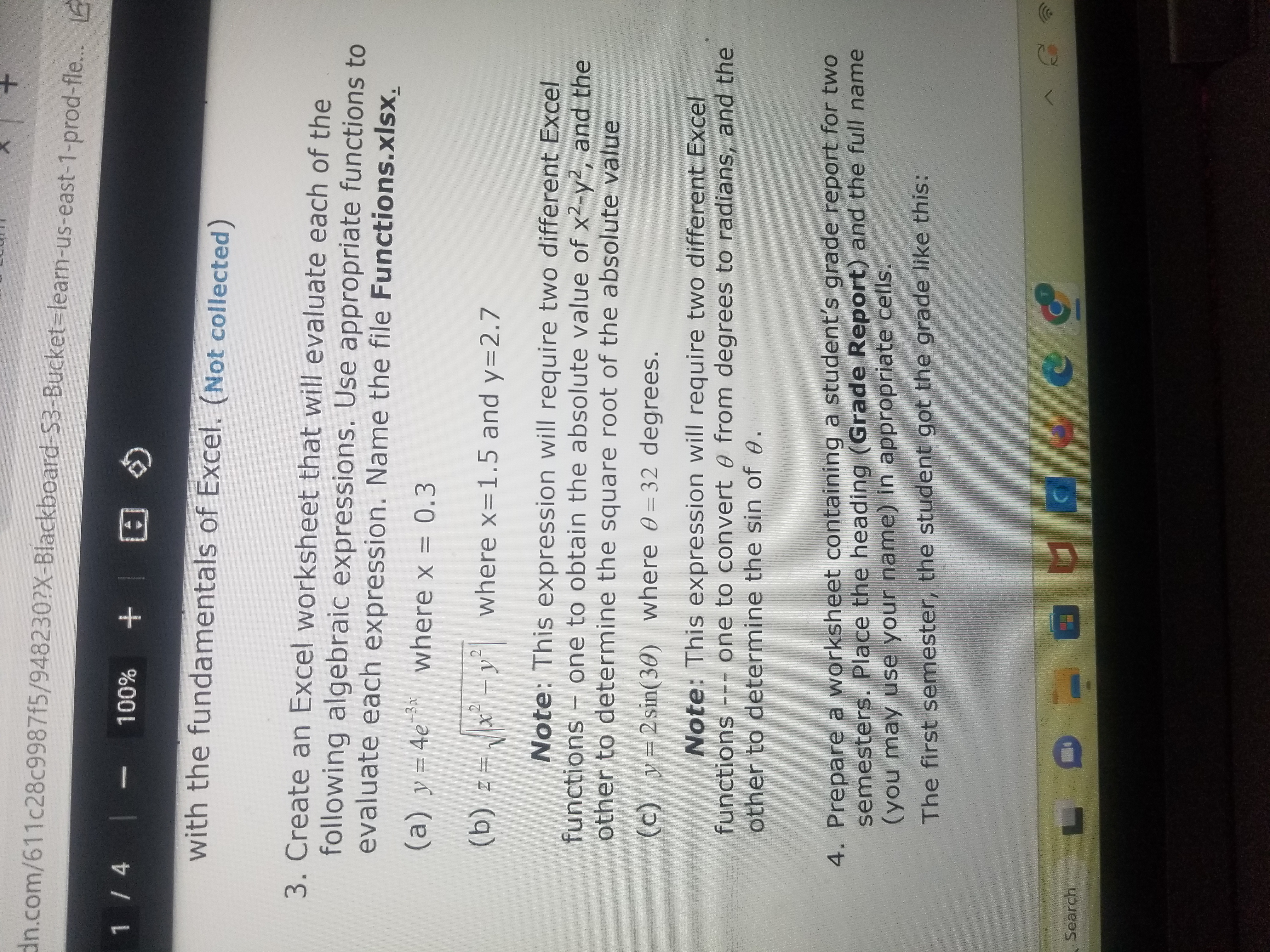
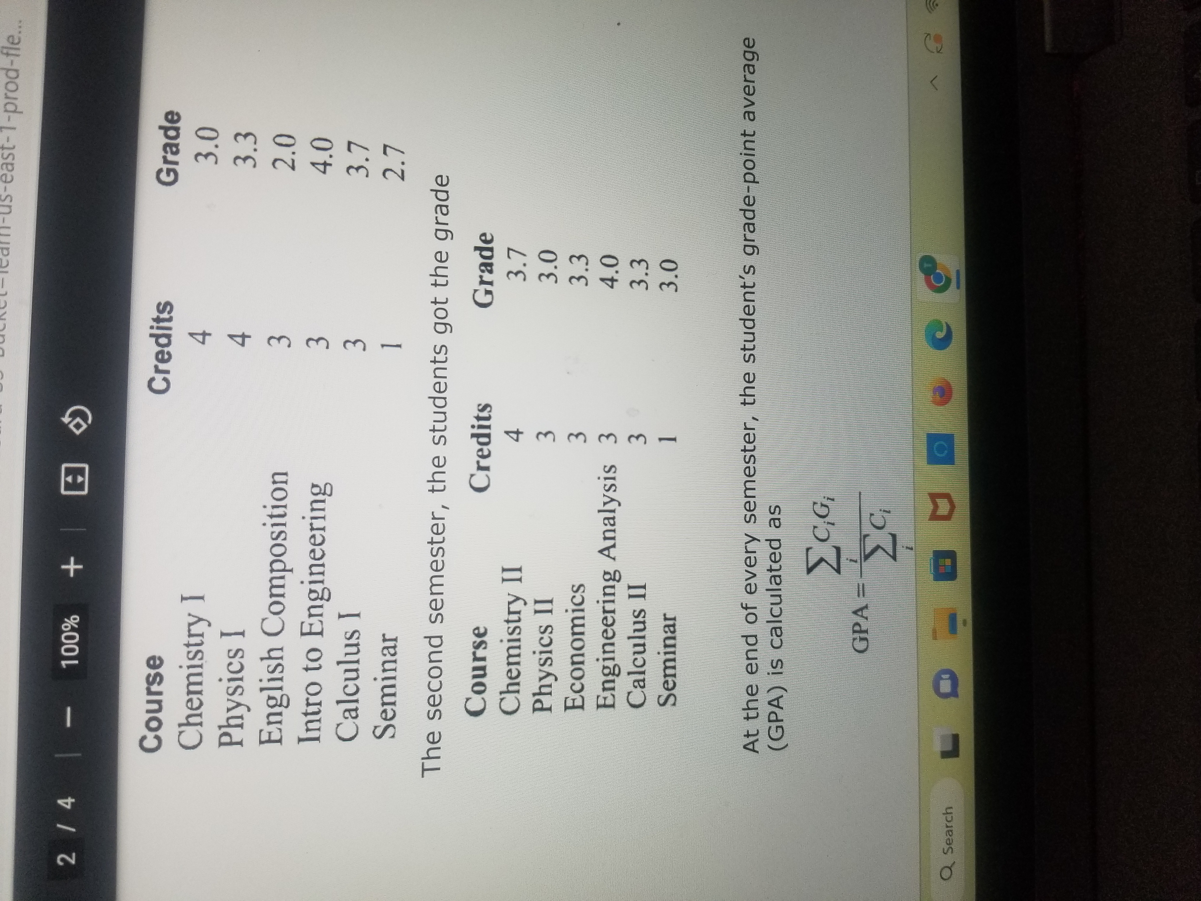
+ cdn.com/611c28c9987f5/948230?X-Blackboard-S3-Bucket-learn-us-east-1-prod-fle... 1/4 |- + 100% + | ED EGR-103 Computer Applications in Engineering Assignment No. 1 * Note that every spreadsheet that you create must have your name in cell A1, the course and section number in cell A2 and the current date in cell A3. All other information will be placed below this regardless of what the problem states. Search 1. Read chapter 1 in the Spreadsheet Tools for Engineers. (Not collected) 2. Read chapter 2 in the Spreadsheet Tools for Engineers. Do all the sample examples illustrated in the text to become proficient with the fundamentals of Excel. (Not collected) 3. Create an Excel worksheet that will evaluate each of the following algebraic expressions. Use appropriate functions to evaluate each expression. Name the file Functions.xlsx. (a) y = 4e3x (b) z = 2 where x = 0.3 x-y where x=1.5 and y=2.7 H Search + dn.com/611c28c9987f5/948230?X-Blackboard-S3-Bucket-learn-us-east-1-prod-fle... 1/4 | - 100% + with the fundamentals of Excel. (Not collected) 3. Create an Excel worksheet that will evaluate each of the following algebraic expressions. Use appropriate functions to evaluate each expression. Name the file Functions.xlsx. -3x (a) y = 4e where x = 0.3 2 x-y| where x=1.5 and y=2.7 (b) = = X Note: This expression will require two different Excel functions one to obtain the absolute value of x-y, and the other to determine the square root of the absolute value (c) y = 2sin(30) where 0=32 degrees. Note: This expression will require two different Excel functions one to convert from degrees to radians, and the other to determine the sin of 0. 4. Prepare a worksheet containing a student's grade report for two semesters. Place the heading (Grade Report) and the full name (you may use your name) in appropriate cells. The first semester, the student got the grade like this: 2/4 | - 100% + Q Search DUCRC-Team-Us-east-1-prod-fle... Course Credits Grade Chemistry I 4 3.0 Physics I 4 3.3 English Composition 3 2.0 Intro to Engineering 3 4.0 Calculus I 3 3.7 Seminar 1 2.7 The second semester, the students got the grade Course Credits Grade Chemistry II 4 3.7 Physics II 3 3.0 Economics 3 3.3 Engineering Analysis 3 4.0 Calculus II 3 3.3 Seminar 1 3.0 At the end of every semester, the student's grade-point average (GPA) is calculated as GPA = C,G < Bb ENGR-203 Bb Courses - Blackboard Learn * + ardcdn.com/611c28c9987f5/948230?X-Blackboard-S3-Bucket-learn-us-east-1-prod-fle... 2/4 | - 100% + (GPA) is calculated as At the end of every semester, the student's grade-point average GPA= CG where C; refers to the number of credits for the ith course and G; refers to the numerical grade for that course. Add a row at the bottom of the worksheet you just created indicating the student's GPA for each semester and the whole school year. Name the file GPA.xlsx. 5. Alice Sloan has just started a marketing research firm called Sloan Research. Her first and only client to date has agreed to pay her $42,000 to conduct a national survey for a new product. Alice will receive payments (revenues) each month for six months: January, $5,000; February, $6,000; March, $7,000; April, $7,000; May, $8,000; and June, $9,000. Q Search A o F9 F10 3: A 1/29 14 - 100% + US-east-1-prod-fle... She has estimated that her monthly expenses during this time period will be: Salaries 2900 Telephone 475 Miscellaneous 110 Rent 735 275 Supplies She also has two periodic expenses. In January, Alice has to prepay a six-month insurance premium of $736. In June, she has a $4,200 small business loan payment due. Create a worksheet using the following steps: a. Enter your name in cell A1, the course and section in cell A2, and the current date in cell A3. b. Enter the worksheet title, Six-Month Budget for Sloan Research, in cell C4 and make the font bold. c. Enter the labels JAN, FEB, MAR, APR, MAY, JUN in cells B5 through G5. They should all be capital letters and right- aligned. Enter TOTAL in cell 15. d. Underline the column headings e. Enter the labels in column A as follows: rch L QQ /611c28c9987f5/948230?X-Blackboard-S3-Bucket-learn-us-east-1-prod-fle... 4 - - 100% + >>> arch e. Enter the labels in column A as follows: Row 6 REVENUES: Row 8 EXPENSES: Row 9 Salaries Row 10 Rent Row 11 Row 12 Telephone Insurance Row 13 Loan Row 14 Supplies Row 15 Misc Row 17 TOTAL EXP: Row 19 NET: Widen column A so that text doesn't overflow into column B f. Enter the values for the monthly revenues (payments) in cells B6 through G6 4 com/611c28c9987f5/948230?X-Blackboard-S3-Bucket-learn-us-east-1-prod-fle... D - 14 | - 100% + Search g. Enter the fixed monthly expenses for January through June. (Remember, insurance and loan payment expenses are periodic and must also be entered.) h. Enter the formula to calculate the Total Revenues in cell 16 i. Alice Sloan forgot to include a local 2.3 percent business tax on revenues. She would like to enter this expense in the row just below Telephone. Insert a row in the appropriate space. Enter the label Local Tax in cell A12. Enter the appropriate formula (0.023 times monthly revenues) in cell B12. Copy this formula from cell B12 to cells C12 through G12 j. Alice has decided that a reserve fund should be created to support the development of new business clients. She thinks that 3 percent of monthly revenues should be put into this fund. Enter the label Reserve in cell A17. Enter the formula to make this calculation in cell B17. Copy this formula across the row through cell G17. Insert a blank row following row 17 k. Use an Excel function to calculate the Total Monthly Expenses in cells B19 through G19. Use formulas to calculate the Net Monthly Income (net=revenue - total expense) in cells B21 through G21 1. Use an Excel function to compute the total for each row in column I T 4 ENGR-203 Bb Courses - Blackboard Learn X + .com/611c28c9987f5/948230?X-Blackboard-S3-Bucket-learn-us-east-1-prod-fle... 4/4 | - 100% + in cells B19 through G19. Use formulas to calculate the Net Monthly Income (net=revenue - total expense) in cells B21 through G21 1. Use an Excel function to compute the total for each row in column I m. After studying the net balances and thinking about the importance of developing new business, Alice decides to increase the percentage allocation to the reserve fund. The current percentage is 3 percent of Revenues. Change the percent used to calculate the reserve fund so that the total Net is as close to, but no less than, $4500, to the nearest dollar. Note that the percentage allocated to the reserve fund must be changed for each month. (The easiest way to do this is to change it for JAN and then use the Copy Command for FEB - JUN.) n. Format the values using currency and no decimal places. This will cause each value to have a "$" printed in front of it and have no decimal places o. Save the worksheet using the filename SLOAN.xlsx Search