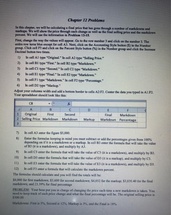
Chapter 12 Problems In this chunpter, we will be calculating a final price that has gone through a number of markdowns and markups. We will show the price through each change as well as the final selling price and the markdown percent. We will use the information in Problem 12-15. First, change the way the values will appear. Go to the row number 3 and click on the number 3. The entire row turns blue except for cell A3. Next, click on the Accounting Style button (5) in the Number group. Click cell F3 and click on the Percent Style button (%) in the Number group and click the Increase Decimal button two times 1) In cell A1 type "Original." In cell A2 type "Selling Price." 2) In cell B1 type "First." In cell B2 type "Markdown." 3) In cell C1 type "Second." In cell C2 type "Markdown." 4) In cell El type "Final." In cell E2 type "Markdown." 5) In cell F1 type "Markdown." In cell F2 type "Percentage." 6) In cell D2 type "Markup." Adjust your columns width and add a bottom border to cells A2:F2. Center the data you typed in A1:52. Your spreadsheet should look like this: C8 D A B 1 Original First Second 2. Selling Price Markdown Markdown 3 Final Markdown Markdown Percentage Markup 7) In cell A3 enter the figure $5,000. 8) Enter the formulas keeping in mind you must subtract or add the percentages given from 100% depending on if it is a markdown or a markup. In cell B3 enter the formula that will take the value of B3 (it is a markdown), and multiply by A3. 9) In cell C3 enter the formula that will take the value of C3 (it is a markdown), and multiply by B3. 10) In cell D3 enter the formula that will take the value of D3 (it is a markup), and multiply by C3. 11) In cell E3 enter the formula that will take the value of 3 (it is a markdown), and multiply by D3. 12) In cell F3 enter a formula that will calculate the markdown percent. The formulas should calculate and you will find the totals will be $4,000 for first markdown: $3,600 for second markdown: $4,032 for the markup: $3,830.40 for the final murkdown; and 23 39% for final percentage PROBLEM: Your bons put you in charge of changing the price each time a new markdown is taken. You need to keep track of each price change and what the final percentage will be. The original selling price is $300.00 Markdown: First is 5%, Second is 12%, Markup is 3%, and the Final is 18% Chapter 12 Problems In this chunpter, we will be calculating a final price that has gone through a number of markdowns and markups. We will show the price through each change as well as the final selling price and the markdown percent. We will use the information in Problem 12-15. First, change the way the values will appear. Go to the row number 3 and click on the number 3. The entire row turns blue except for cell A3. Next, click on the Accounting Style button (5) in the Number group. Click cell F3 and click on the Percent Style button (%) in the Number group and click the Increase Decimal button two times 1) In cell A1 type "Original." In cell A2 type "Selling Price." 2) In cell B1 type "First." In cell B2 type "Markdown." 3) In cell C1 type "Second." In cell C2 type "Markdown." 4) In cell El type "Final." In cell E2 type "Markdown." 5) In cell F1 type "Markdown." In cell F2 type "Percentage." 6) In cell D2 type "Markup." Adjust your columns width and add a bottom border to cells A2:F2. Center the data you typed in A1:52. Your spreadsheet should look like this: C8 D A B 1 Original First Second 2. Selling Price Markdown Markdown 3 Final Markdown Markdown Percentage Markup 7) In cell A3 enter the figure $5,000. 8) Enter the formulas keeping in mind you must subtract or add the percentages given from 100% depending on if it is a markdown or a markup. In cell B3 enter the formula that will take the value of B3 (it is a markdown), and multiply by A3. 9) In cell C3 enter the formula that will take the value of C3 (it is a markdown), and multiply by B3. 10) In cell D3 enter the formula that will take the value of D3 (it is a markup), and multiply by C3. 11) In cell E3 enter the formula that will take the value of 3 (it is a markdown), and multiply by D3. 12) In cell F3 enter a formula that will calculate the markdown percent. The formulas should calculate and you will find the totals will be $4,000 for first markdown: $3,600 for second markdown: $4,032 for the markup: $3,830.40 for the final murkdown; and 23 39% for final percentage PROBLEM: Your bons put you in charge of changing the price each time a new markdown is taken. You need to keep track of each price change and what the final percentage will be. The original selling price is $300.00 Markdown: First is 5%, Second is 12%, Markup is 3%, and the Final is 18%


