chapter3: adaptive control

2nd edition

by: karl johan strm bjrn wittenmark

here the problem:

and here, example 3.5

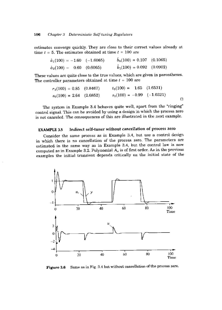
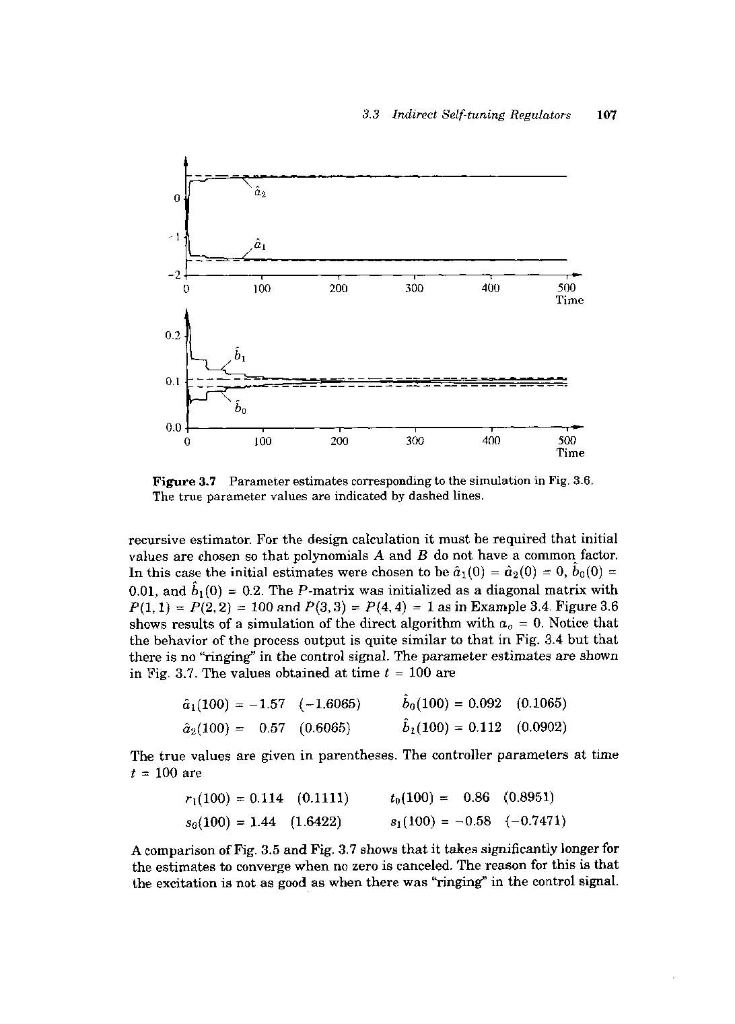
Consider the indirect self-tuning regulator in Example 3.5. Change the specifications on the closed-loop system, and investigate how the behavior of the system changes. 106 Chapter 3 Deterministie Self-tuning Regulators estimates converge quickly. They are close to their correct values already at time t = 5. The estimates obtained at time t = 100 are (100) = -1.60 (-1.6065) bo(100) = 0.107 (0.1065) 62(100) = 0.60 (0.6065) b(100) = 0.092 (0.0902) These values are quite close to the true values, which are given in parentheses. The controller parameters obtained at time t - 100 are (100) = 0.85 (0.8467) to(100) 1.65 (1.6531) So(100) = 2.64 (2.6852) 8 (100) = -0.99 (-1.0321) The system in Example 3.4 behaves quite well, apart from the "ringing" control signal. This can be avoided by using a design in which the process zero is not canceled. The consequences of this are illustrated in the next example. EXAMPLE 3.5 Indirect self-tuner without cancellation of process zero Consider the same process as in Example 3.4, but use a control design in which there is no cancellation of the process zero. The parameters are estimated in the same way as in Example 3.4, but the control law is now computed as in Example 3.2. Polynomial A, is of first order. As in the previous examples the initial transient depends critically on the initial state of the 119 Time Figure 3.6 Same as in Fig. 3.4 but without cancellation of the process zero. 3.3 Indirect Self-tuning Regulators 107 a 100 200 200 300 400 500 Time 0.1- 0.0 100 200 300 400 500 Time Figure 3.7 Parameter estimates corresponding to the simulation in Fig. 3.6. The true parameter values are indicated by dashed lines. recursive estimator. For the design calculation it must be required that initial values are chosen so that polynomials A and B do not have a common factor In this case the initial estimates were chosen to be a,(0) = 2(0) - 0, bo(0) - 0.01, and b (0) = 0.2. The P-matrix was initialized as a diagonal matrix with P(1.1) = P(2.2) = 100 and P(3,3) = P(4, 4) = 1 as in Example 3.4. Figure 3.6 shows results of a simulation of the direct algorithm with = 0. Notice that the behavior of the process output is quite similar to that in Fig. 3.4 but that there is no "ringing" in the control signal. The parameter estimates are shown in Fig. 3.7. The values obtained at time t = 100 are ai(100) = -1.57 (-1.6065) Po(100) = 0.092 (0.1065) @y(100) - 0.57 (0.6065) 62(100) = 0.112 (0.0902) The true values are given in parentheses. The controller parameters at time t = 100 are n(100) = 0.114 (0.1111) to(100) = 0.86 0.8951) so(100) = 1.44 (1.6422) 8,(100) = -0.58 (-0.7471) A comparison of Fig. 3.5 and Fig. 3.7 shows that it takes significantly longer for the estimates to converge when no zero is canceled. The reason for this is that the excitation is not as good as when there was "ringing in the control signal. 108 Chapter 3 Deterministic Self-tuning Regulators There is very little excitation of the system in the periods when the output and the control signals are constant. This explains the steplike behavior of the estimates. It may seem surprising that the controller already gives the correct steady- state value at timet - 20 when the parameter estimates differ so much from their correct values. The controller parameters are r (20) = 0.090 (0.1111) to(20) - 0.83 (0.8951) 80 (20) = 1.13 (1.6422) S (20) = -0.29 (-0.7471) Since the process has integral action, we have A(1) - 0. It then follows from Eq. (3.3) that the static gain from command signal to output is B(1)T(1) T(1) A(1)R(1) + B(1)S(1) S(1) To obtain the correct steady-state value, it is thus sufficient that the controller parameters are such that S(1) = T(1), which in the special case is the same as to - 80 + 81. When no poles are canceled, it follows from Eq. (3.12) that T(1) = A (1)B(1) = A (1) An (1) B (1) where B is the estimated B polynomial. Hence T(1) A.(1)A. (1) - 1 S(1) B(1)S(1) where the last equality follows from Eq. (3.11). Notice that we have A(1) = 0. We thus obtain the rather surprising conclusion that the adaptive controller in this case will automatically have parameters such that there will be no steady-state error. These examples indicate that the indirect self-tuning algorithm behaves as can be expected and that the estimate of convergence time given by Eq. (3.23) is reasonable. The examples also show the importance of using a good un- derlying control design. With model-following design it is recommended that cancellation of process zeros is avoided. Summary The indirect self-tuning regulator based on model-following given by Algo- rithm 3.1 is a straightforward application of the idea of self-tuning. The adap- tive controller has states that correspond to the parameter estimate y, the covariance matrix P, the regression vectory, and the states required for the implementation of the control law. The controller in Example 3.4 has 20 state variables, updating of the covariance matrix P alone requires ten states. The Consider the indirect self-tuning regulator in Example 3.5. Change the specifications on the closed-loop system, and investigate how the behavior of the system changes. 106 Chapter 3 Deterministie Self-tuning Regulators estimates converge quickly. They are close to their correct values already at time t = 5. The estimates obtained at time t = 100 are (100) = -1.60 (-1.6065) bo(100) = 0.107 (0.1065) 62(100) = 0.60 (0.6065) b(100) = 0.092 (0.0902) These values are quite close to the true values, which are given in parentheses. The controller parameters obtained at time t - 100 are (100) = 0.85 (0.8467) to(100) 1.65 (1.6531) So(100) = 2.64 (2.6852) 8 (100) = -0.99 (-1.0321) The system in Example 3.4 behaves quite well, apart from the "ringing" control signal. This can be avoided by using a design in which the process zero is not canceled. The consequences of this are illustrated in the next example. EXAMPLE 3.5 Indirect self-tuner without cancellation of process zero Consider the same process as in Example 3.4, but use a control design in which there is no cancellation of the process zero. The parameters are estimated in the same way as in Example 3.4, but the control law is now computed as in Example 3.2. Polynomial A, is of first order. As in the previous examples the initial transient depends critically on the initial state of the 119 Time Figure 3.6 Same as in Fig. 3.4 but without cancellation of the process zero. 3.3 Indirect Self-tuning Regulators 107 a 100 200 200 300 400 500 Time 0.1- 0.0 100 200 300 400 500 Time Figure 3.7 Parameter estimates corresponding to the simulation in Fig. 3.6. The true parameter values are indicated by dashed lines. recursive estimator. For the design calculation it must be required that initial values are chosen so that polynomials A and B do not have a common factor In this case the initial estimates were chosen to be a,(0) = 2(0) - 0, bo(0) - 0.01, and b (0) = 0.2. The P-matrix was initialized as a diagonal matrix with P(1.1) = P(2.2) = 100 and P(3,3) = P(4, 4) = 1 as in Example 3.4. Figure 3.6 shows results of a simulation of the direct algorithm with = 0. Notice that the behavior of the process output is quite similar to that in Fig. 3.4 but that there is no "ringing" in the control signal. The parameter estimates are shown in Fig. 3.7. The values obtained at time t = 100 are ai(100) = -1.57 (-1.6065) Po(100) = 0.092 (0.1065) @y(100) - 0.57 (0.6065) 62(100) = 0.112 (0.0902) The true values are given in parentheses. The controller parameters at time t = 100 are n(100) = 0.114 (0.1111) to(100) = 0.86 0.8951) so(100) = 1.44 (1.6422) 8,(100) = -0.58 (-0.7471) A comparison of Fig. 3.5 and Fig. 3.7 shows that it takes significantly longer for the estimates to converge when no zero is canceled. The reason for this is that the excitation is not as good as when there was "ringing in the control signal. 108 Chapter 3 Deterministic Self-tuning Regulators There is very little excitation of the system in the periods when the output and the control signals are constant. This explains the steplike behavior of the estimates. It may seem surprising that the controller already gives the correct steady- state value at timet - 20 when the parameter estimates differ so much from their correct values. The controller parameters are r (20) = 0.090 (0.1111) to(20) - 0.83 (0.8951) 80 (20) = 1.13 (1.6422) S (20) = -0.29 (-0.7471) Since the process has integral action, we have A(1) - 0. It then follows from Eq. (3.3) that the static gain from command signal to output is B(1)T(1) T(1) A(1)R(1) + B(1)S(1) S(1) To obtain the correct steady-state value, it is thus sufficient that the controller parameters are such that S(1) = T(1), which in the special case is the same as to - 80 + 81. When no poles are canceled, it follows from Eq. (3.12) that T(1) = A (1)B(1) = A (1) An (1) B (1) where B is the estimated B polynomial. Hence T(1) A.(1)A. (1) - 1 S(1) B(1)S(1) where the last equality follows from Eq. (3.11). Notice that we have A(1) = 0. We thus obtain the rather surprising conclusion that the adaptive controller in this case will automatically have parameters such that there will be no steady-state error. These examples indicate that the indirect self-tuning algorithm behaves as can be expected and that the estimate of convergence time given by Eq. (3.23) is reasonable. The examples also show the importance of using a good un- derlying control design. With model-following design it is recommended that cancellation of process zeros is avoided. Summary The indirect self-tuning regulator based on model-following given by Algo- rithm 3.1 is a straightforward application of the idea of self-tuning. The adap- tive controller has states that correspond to the parameter estimate y, the covariance matrix P, the regression vectory, and the states required for the implementation of the control law. The controller in Example 3.4 has 20 state variables, updating of the covariance matrix P alone requires ten states. The