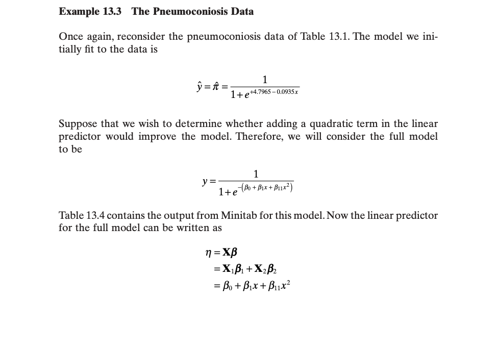
Check if adding a quadratic term in the regressor improves the model. Refer to the example below.
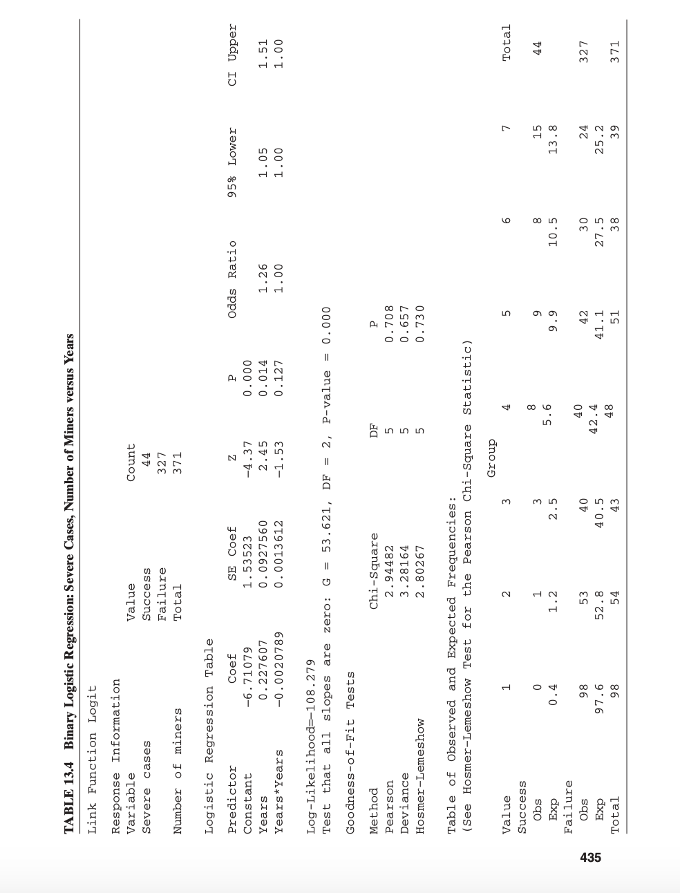
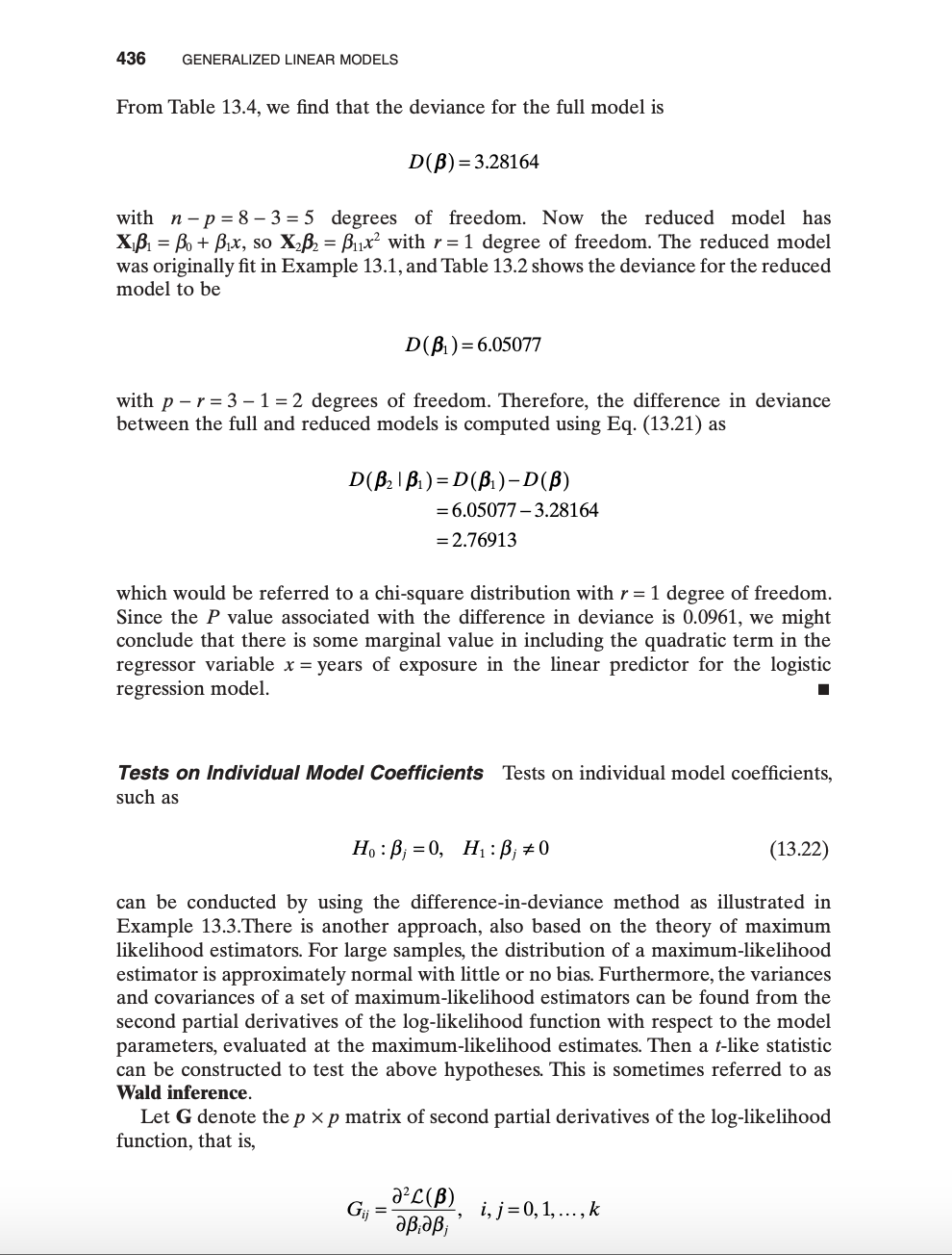
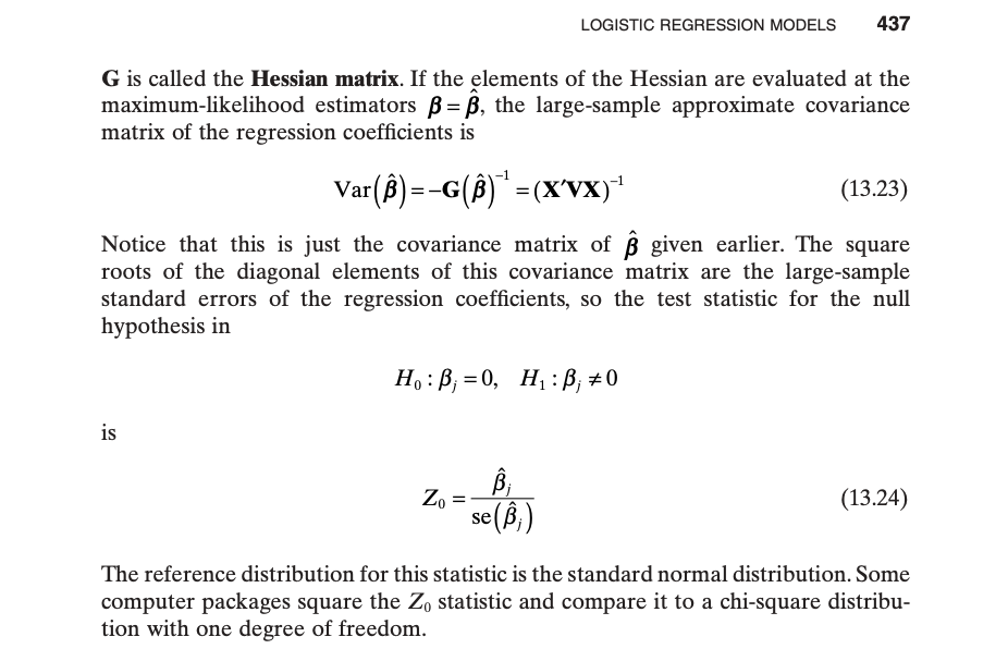
Example 13.3 The Pneumoconiosis Data Once again, reconsider the pneumoconiosis data of Table 13.1. The model we ini- tially fit to the data is y= 1 =- 1 1 + e+4.7965 -0.0935x Suppose that we wish to determine whether adding a quadratic term in the linear predictor would improve the model. Therefore, we will consider the full model to be y= Ite (Bo + Bix + Blix2) Table 13.4 contains the output from Minitab for this model. Now the linear predictor for the full model can be written as n = XB =XiBi+ X2Bz = Bo + Bix+ Blix2TABLE 13.4 Binary Logistic Regression: Severe Cases, Number of Miners versus Years Link Function Logit Response Information Variable Value Count Severe cases Success 44 Failure 327 Number of miners Total 371 Logistic Regression Table Predictor Coef SE Coef N Odds Ratio 95% Lower CI Upper Constant -6. 71079 1. 53523 -4.37 0. 000 Years 0. 227607 0 . 0927560 2.45 0 . 014 1.26 1 . 05 1 .51 Years*Years -0 . 0020789 0 . 0013612 -1.53 0. 127 1. 00 1.00 1. 00 Log-Likelihood=-108.279 Test that all slopes are zero: G = 53.621, DF = 2, P-value = 0. 000 Goodness-of-Fit Tests Method Chi-Square DF Pearson 2. 94482 0 . 708 Deviance 3. 28164 0 . 657 Hosmer-Lemeshow 2 . 80267 In in in 0. 730 Table of Observed and Expected Frequencies: (See Hosmer-Lemeshow Test for the Pearson Chi-Square Statistic) Group Value m Total Success Obs O 15 Exp 0.4 H m in 13 . 8 Failure 40 435 Obs 86 24 327 Exp 97 . 6 52 . 8 40.5 42 .4 41. 1 in 25 .2 Total 98 38 39 371436 GENERALIZED LINEAR MODELS From Table 13.4, we nd that the deviance for the full model is 13(3): 3.28164 with n p = 8 3 = 5 degrees of freedom. Now the reduced model has XIl = , + lx, so X232 = uxz with r = 1 degree of freedom. The reduced model was originally t in Example 13.1, and Table 13.2 shows the deviance for the reduced model to be D(1)=6.05077 with p r = 3 1 = 2 degrees of freedom. Therefore, the difference in deviance between the full and reduced models is computed using Eq. (13.21) as DUE |1)=D(1)-D() =6.050?7 3.28164 = 2.76913 which would be referred to a chi-square distribution with r = 1 degree of freedom. Since the P value associated with the difference in deviance is 0.0961, we might conclude that there is some marginal value in including the quadratic term in the regressor variable x =years of exposure in the linear predictor for the logistic regression model. I Tests an Individual Made! Coefcients Tests on individual model coefcients, such as HI] : ! =0, H1Ij in (13.22) can be conducted by using the difference-in-deviance method as illustrated in Example 13.3.There is another approach, also based on the theory of maximum likelihood estimators. For large samples, the distribution of a maximum-likelihood estimator is approximately normal with little or no bias. Furthermore, the variances and covariances of a set of maximum-likelihood estimators can be found from the second partial derivatives of the log-likelihood function with respect to the model parameters, evaluated at the maximum-likelihood estimates. Then a Hike statistic can be constructed to test the above hypotheses. This is sometimes referred to as Wald inference. Let G denote the p x p matrix of second partial derivatives of the log-likelihood function, that is, amt!) . . ..= , =0,1....,k G\" aia.' \" LOGISTIC REGRESSION MODELS 437 G is called the Hessian matrix. If the elements of the Hessian are evaluated at the maximum-likelihood estimators B =B, the large-sample approximate covariance matrix of the regression coefficients is Var( B) =-G(B) =(X'VX)" (13.23) Notice that this is just the covariance matrix of B given earlier. The square roots of the diagonal elements of this covariance matrix are the large-sample standard errors of the regression coefficients, so the test statistic for the null hypothesis in Ho : B, =0, H1 :B, #0 is Zo = se ( B,) (13.24) The reference distribution for this statistic is the standard normal distribution. Some computer packages square the Zo statistic and compare it to a chi-square distribu- tion with one degree of freedom
