!Clearly solve the following.

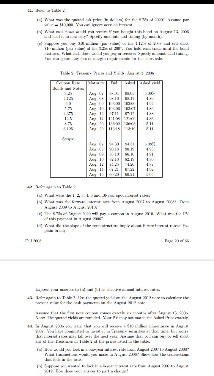
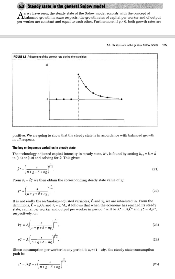
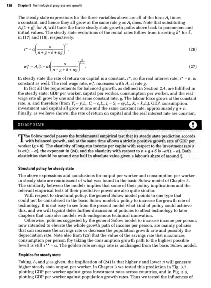
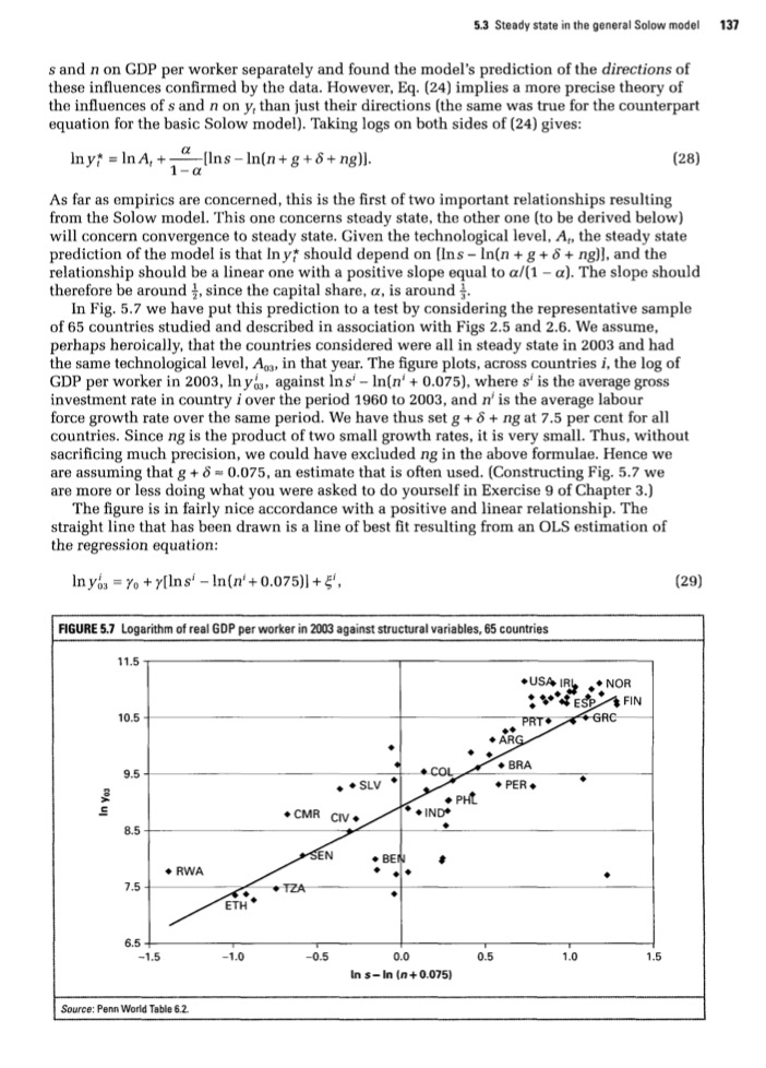
41. Refer to Table 2. {a} What was the quoted ask price (in dollars] for the 8.753 of 2020'? Assume par value = $10,000. You can ignore accrued interest. (b) What cash ows would you receive ifyou bought this bond on August 13, 2006 and held it to maturity? Specify mounts and timing {by month]. (c) Suppose you buy 310 million (par value) of the 4.125s of 2008 and sell short $10 million [par value} of the 3.255 of 212m. You hold each trade until the bend matures. What cash ows would you pay or receive? Specify amounts and timing. You can ignore any fees or margin requirements for the short sale. Table 2: Treasury Prices and Yields, August 3. 2006 Inl Ashamed Bonds and Notes: 3. 25 4 .125 5. 0 5. 75 4 3T5 l 2.5 3. 75 6 .125 Stripe: 42. Refer again to Table 2. {a} What were the l._ 2, 3, 4. 6 and 10-year soot interest rates? {b} What was the forward interest rate from August 2(1)? to August 2008'? From August m to August 2010'? (c) The 8.753 of August 2020 will pay a coupon in August 2010. What was the PV of this payment in August. 2113'? [d] iJirl'llat did the slope of the term structure imply about future interest rates? Ex- plain briey. Fall 2008 Page 20 of 63 Express your answers to (a) and (b) as effective annual interest rates. 43. Refer again to Table 2. Use the quoted yield on the August 2012 note to calculate the present value for the cash payments on the August 2012 note. AsSume that the rst note coupon comes exactly six months after August 13. 2006. Note: The quoted yields are rounded. Your PV may not match the Asked Price exactly. 44. In August 2006 you learn that you will receive a $10 million inheritance in August 2111?. You have committed to invest it in 'Il-easury securities at that tinie. but worry that interest rates may [all over the next year. Assume that you can buy or sell short any of the Treasuries in Table 2 at the prices listed in the table. {a} How would you lock in a one-year interest rate from August 2007 to August 2W3? What transactions would you make in August 2000'? Show how the transactions that lock in the rate. (b) Suppose you wanted to lock in a 5-year interest rate from August 2007 to August 3012'. How does your answer to part a change? Exercise 9. Where growth comes from according to tho Solow model and according to growth accounting Assume that some economy behaves completely in accordance with the steady state of the Solow model presented in this chapter, where the assumed growth rate of A: is g. From what you have learned in this chapter, what will the average annual growth rates of Yr: k, and A, be over some period from year tto year T? What creates growth in GDP per worker? If one did a growth accounting exercise for this economy, what would be the fractions of growth in GDP per worker attributed to growth in capital per worker and to growth in At, respectively? Again, what is the true source of growth in this economy? Steady state in the general Solow model s we have seen, the steady state of the Solow model accords with the concept of Abalanced growth in some respects: the growth rates of capital per worker and of output per worker are constant and equal to each other. Furthermore, if g > 0, both growth rates are 5.3 Steady state in the general Solow model 135 FIGURE 5.6 Adjustment of the growth rate during the transition positive. We are going to show that the steady state is in accordance with balanced growth in all respects. The key endogenous variables in steady state The technology-adjusted capital intensity in steady state, k*, is found by setting k,. = k, = in (16) or (19) and solving for K. This gives: K* = S (21) In+g+8+ng From y, = k, we then obtain the corresponding steady state value of y; * = S (22) n+g+6+ng It is not really the technology-adjusted variables, k, and y,, we are interested in. From the definitions, k, = k,/A, and y, = y,/A,, it follows that when the economy has reached its steady state, capital per worker and output per worker in period : will be k* = A,K* and y; = Ajj*, respectively, or: K* = A, S (23) in+g+o+ng y* = A S (24) n+g+o+ng Since consumption per worker in any period is c, = (1 - sly,, the steady state consumption path is: C* = A,(1 - s) S (25) n+g+o+ng136 Chapter 5 Technological progress and growth The steady state expressions for the three variables above are all of the form A, times a constant, and hence they all grow at the same rate g as A, does. Note that substituting A.(1 + g)' for A, will trace the three steady state growth paths above back to parameters and initial values. The steady state evolutions of the rental rates follow from inserting k* for k, in (17) and (18), respectively: r* = a S (26) (n+g+6+ng) w; = A,(1 - a) (27) n+g+6+ng In steady state the rate of return on capital is a constant, r*, so the real interest rate, r* - 8, is constant as well. The real wage rate, w,, increases with A, at rate g. In fact all the requirements for balanced growth, as defined in Section 2.4, are fulfilled in the steady state: GDP per worker, capital per worker, consumption per worker, and the real wage rate all grow by one and the same constant rate, g. The labour force grows at the constant rate, n, and therefore (from Y, = y,L, C, = C,L, I, = S, = sy,L,. K, = k,L,), GDP, consumption, investment and capital all grow at one and the same constant rate, approximately g + n. Finally, as we have shown, the rate of return on capital and the real interest rate are constant. STEADY STATE O The Solow model passes the fundamental empirical test that its steady state prediction accords with balanced growth, and at the same time allows a strictly positive growth rate of GDP per worker (g > 0). The elasticity of long-run income per capita with respect to the investment rate s is a/(1 - a), the exponent in (24), and the elasticity with respect to n + g +6 is -a/(1 - a). Both elasticities should be around one half in absolute value given a labour's share of around }. Structural policy for steady state The above expressions and conclusions for output per worker and consumption per worker in steady state are reminiscent of what was found in the basic Solow model of Chapter 3. The similarity between the models implies that some of their policy implications and the relevant empirical tests of their predictive power are also quite similar. With respect to structural policy, the general Solow model points to one type that could not be considered in the basic Solow model: a policy to increase the growth rate of technology. It is not easy to see from the present model what kind of policy could achieve this, and we will (again) defer further discussion of policies to affect technology to later chapters that consider models with endogenous technical innovation. Otherwise, policies suggested by the general Solow model to increase income per person, now intended to elevate the whole growth path of income per person, are mainly policies that can increase the savings rate or decrease the population growth rate and possibly the depreciation rate. Note also from (25) that the value of the savings rate that maximizes consumption per person (by taking the consumption growth path to the highest possible level) is still s** = a. The golden rule savings rate is unchanged from the basic Solow model. Empirics for steady state Taking A, and gas given, the implication of (24) is that higher s and lower n will generate higher steady state output per worker. In Chapter 3 we tested this prediction in Fig. 3.7, plotting GDP per worker against gross investment rates across countries, and in Fig. 3.8, plotting GDP per worker against population growth rates. Thus we tested the influences ofa: Main innit- casual seine model s and n on GDP per worker separater and found the model's prediction of the directions of these inuences confirmed by the data. However. Eq. [24] implies a more precise theory of the inuences of s and n on y. than just their directions [the same was true for the counterpart equation for the basic Solow model]. Thking logs on both sides of [24] gives: lnyf' - ina.+uns-ln[n+g+s+ngn. [as] As Far as empirics are concerned. this is the rst of two important relationships resulting from the Solow model. This one concerns steady state. the other one [to be derived below} will concern convergence to steady state. Given the technological level. at... the steady state prediction of the model is that In yr should depend on [ins - lnin + g+ s e 113]]. and the relationship Shetd he a linear one with a positive slope equal to still - a]. The slope should therefore be around 1}. since the capital share. tr. is around 1}. in Fig. 5.? we have put this prediction to a test by considering the representative sample of as countries studied and described in association with Figs 2.! and 2.5. We assume. perhaps heroically. that the countries considered were all in steady state in 20113 and had the same technological level. An... in that year. The gure plots. across countries 1'. the log of GDP per worker in EDGE. lltyll\". against lns' - lnljni + 0.0%}. where s'r is the aver-age gross lnvestrnent rate in country i ever the period 19m to 2003. and n" is the average labour force growth rate over the same period. We have thus set g + s + ng at 11.5 per cent for all countries. Since ng is the product oi" two small growth rates. it is very small. Thus. without sacricing much precision. we could have excluded ng in the above liormulae. Hence we are assuming that g + s - 0.0?5. an estimate that is oeu used. [Constructing Fig. 5.7 we are more or less doing what you were asked to do yourself in Exercise e oi\" Chapter 3.] The gure is in fairly nice accordance with a positive and linear relationship. The straight line that has been drawn is a line of best t resulting from an Dis estimation of the regression equation: lny, =y +y[ins" -ln[n'+tl.tl?5]i+'. [29] Hill: IJ' inquires HHENMWHMWWHMEW hehie-uI-om 138 Chapter 5 Technological progress and growth where 5' is a random error term representing the influence of omitted variables (if necessary, consult the appendix on regression analysis regarding distributional assumptions on 5' etc.). The details of the estimation are: In yaa = 8.92+ 1.52 [Ins' -In(n' + 0.75)]. R' = 0.64, [se=0.14.1=10.5) The estimate of y, the slope of the line, is 1.52. This slope is considerably larger than the 0.5 it should be according to our theory. Note that the standard error of the estimate of y is 0.14. The 95 per cent confidence interval for the estimate goes approximately from two standard deviations below to two standard deviations above the estimate of y, giving a confidence interval of [1.24; 1.80]. This is not close to including the value 0.5, so the estimated slope is significantly larger than 0.5. In fact, for the fraction a/(1 - a) to equal 1.52, a would have to be 0.6. An a of around 0.6 is way above the capital share (around ;) that a should correspond to.' STEADY STATE AND THE CROSS-COUNTRY EMPIRICAL EVIDENCE The steady state of the Solow model matches cross-country data quite well (even under an assumption of a common technological level): there is a clear positive correlation between Iny' and Ins' - In(n' + 0.75) as predicted, and the linear form of the relationship is in nice accordance with the data. However, the model considerably underestimates the strength of the influences of the key parameters on GDP per person compared to the correlation found in the data. The nice positive correlation in Fig. 5.7 is reassuring for our model, but it does not prove that the model's prediction of a positive long-run influence of the investment rate on income per capita is correct. In empirical analysis one must be careful not to confuse correlation with causation and about what is exogenous and what is endogenous. For instance, the picture would be consistent with a reversed causality where the exogenous variable was income per capita, the endogenous variable was the investment rate net of labour force growth, and income per capita had a positive influence on the investment rate net of labour force growth, perhaps through reducing population growth. It could also be spurious correlation, where there would be no causal relationship between the two in any direction, both would be endogenous, and a third exogenous factor, the 'entrepreneurial spirit" of a society, say, influenced both. Assume that entrepreneurial spirit is exogenous and affects both the investment rate and income per capita positively. Then more 'entrepreneurial' societies would tend to have higher investment rates and higher incomes per capita, so a positive correlation between the two would be observed without any causation between them. It may be, in fact, that there is indeed a positive influence of the investment rate net of labour force growth on income per worker and a positive influence of income per capita on the investment rate net of labour force growth and third factors influencing both systematically. In that case a picture like Fig. 5.7 will involve many different forces and viewed as a picture expressing the influence of the investment rate net of labour force growth on income per capita it will be highly distorted. For now, just pick up that there is always a danger of misinterpreting correlation as causality. The positive correlation between the number of policemen and crime rates observed in many countries does not necessarily mean that more policemen imply more crime. It could be a simple reflection that more crime calls for more police. 3. The 95 per cent confidence interval for the implied a is [0.55; 0.64]. Show this