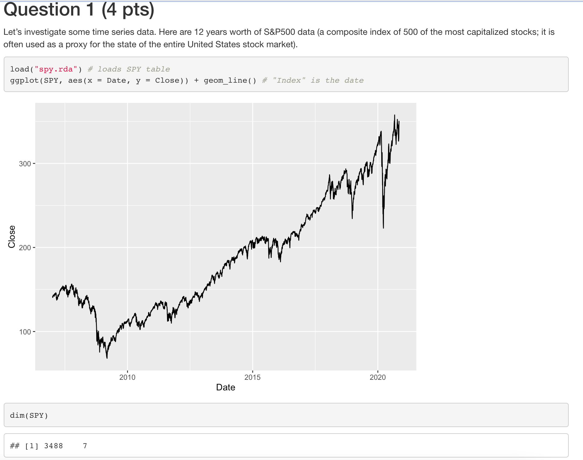
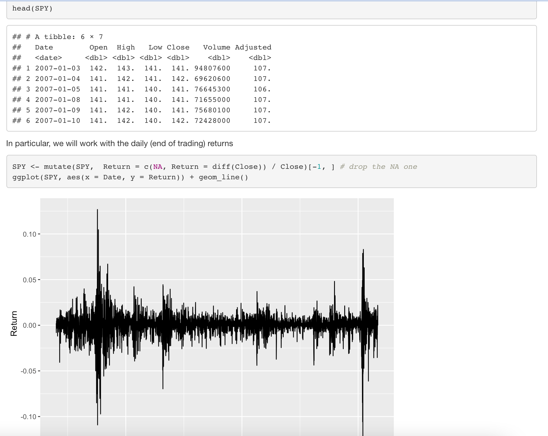
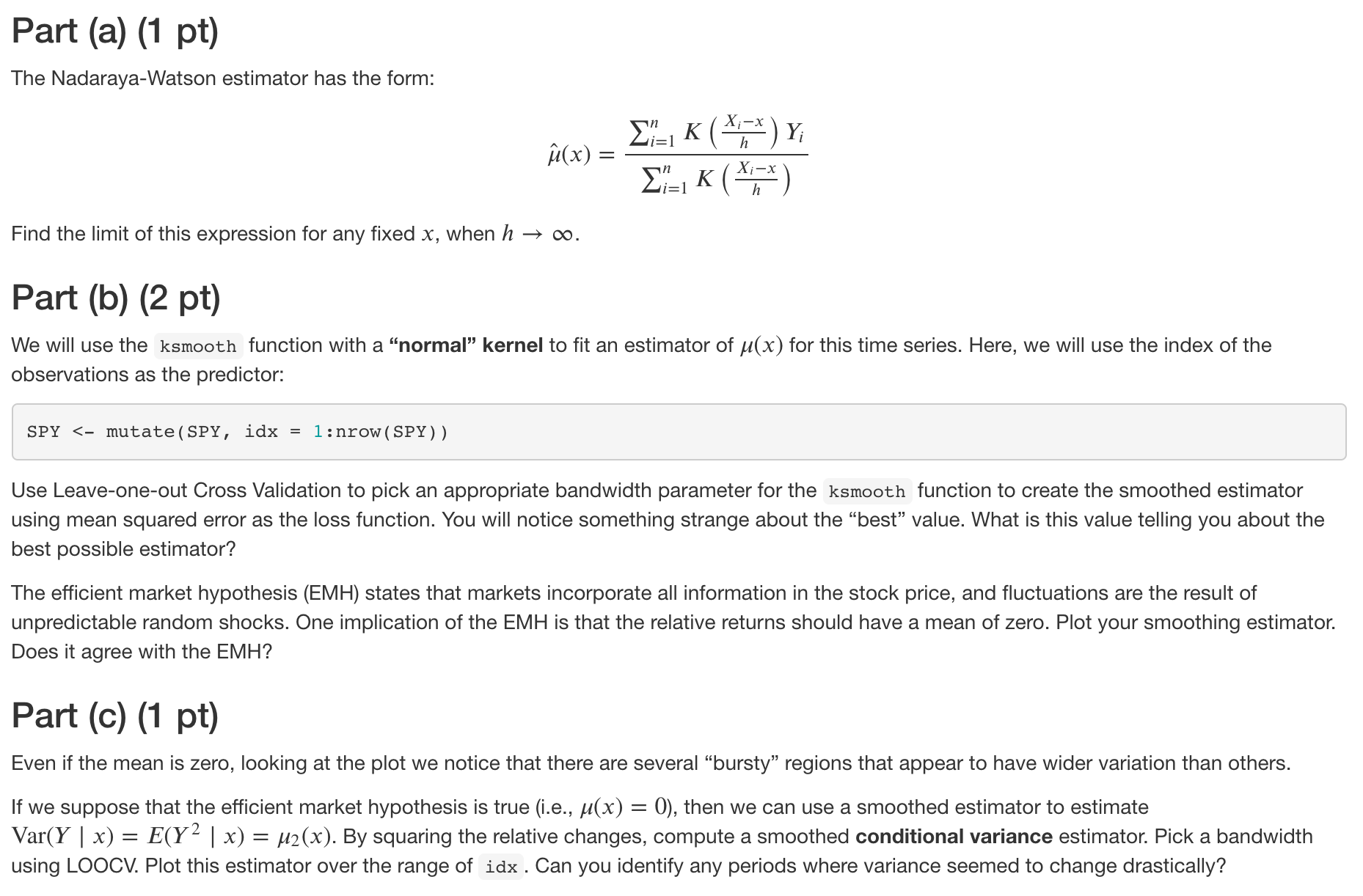
Close Question 1 (4 pts) Let's investigate some time series data. Here are 12 years worth of S&P500 data (a composite index of 500 of the most capitalized stocks; it is often used as a proxy for the state of the entire United States stock market). load("spy.rda") # loads SPY table ggplot (SPY, aes(x = Date, y = Close)) + geom_line() # "Index" is the date 300- 200- 100- dim(SPY) ## [1] 3488 7 20'10 2015 2020 Date Return head (SPY) #23 #23 #3 A tibble: 6 7 ## ## Date Open High Low Close Volume Adjusted ## 1 2007-01-03 142. 143. 141. ## 2 2007-01-04 141. ## 3 2007-01-05 141. ## 4 2007-01-08 141. 141. 140. 141. 71655000 ## 5 2007-01-09 141. 142. 140. 141. 75680100 ## 6 2007-01-10 141. 142. 140. 142. 72428000 141. 94807600 107. 142. 141. 141. 142. 69620600 107. 140. 141. 76645300 106. 107. 107. 107. In particular, we will work with the daily (end of trading) returns SPY < mutate (SPY, Return = c(NA, Return = diff (Close)) / Close) [-1, ] # drop the NA one ggplot (SPY, aes(x = Date, y = Return)) + geom_line( ) 0.10- 0.05- 0.00 - -0.05- -0.10- Part (a) (1 pt) The Nadaraya-Watson estimator has the form: K(xx)Y Y h (x) = K(x-x) h Find the limit of this expression for any fixed x, when h . Part (b) (2 pt) We will use the ksmooth function with a "normal" kernel to fit an estimator of (x) for this time series. Here, we will use the index of the observations as the predictor: SPY