Code posted below

clear all

L=2.; % domain length

%

%need N>3 for it to run

N=20; % number of grid cells

dx=L/N;

dx2=dx^2;

epsilon=0.25;

eps=epsilon^1.333; % the diffusion coefficient is corrected by porosity raised to the 1.33 power

D_O2=1.94e-5; %O2 diffusion in air

D_O2=eps*D_O2; %O2 diffusion in air corrected for porosity

D_CO2=1.51e-5; %CO2 diffusion in air

D_CO2=eps*D_CO2; %CO2 diffusion in air corrected for porosity

k_c=6.99e-6; %reaction rate for oxygen consumption during organic degradation (1/s)

k_cp=k_c*epsilon; %reaction rate corrected for porosity

alf=1.0; %stochiometric coefficient for organics and O_2 to CO_2

%k_h=1e-2; %convection coefficient (m/s)

c_O2_inf=8.2; %molar concentration of O2 in atmospher (m/m^3)

c_CO2_inf=0.0108; %molar concentration of CO2 in atmospher (m/m^3)

c_O2_b=c_O2_inf; % setting boundary concentration for O2 to the ambient value

c_CO2_b=c_CO2_inf; % setting boundary concentration for CO2 to the ambient value

m=sqrt(k_cp/D_O2); % this is the value of 'm' that appears in the case of the 'fin' solution

%

% oxygen solution

%

for i=1:N+1

for j=1:N+1

A(i,j)=0.0;

end

end

%set up the matrix

A(1,1)=1;

A(1,2)=0.0;

A(N+1,N)=-2.0;

A(N+1,N+1)=2.+k_cp*dx2/D_O2;

for i=2:N

A(i,i-1)=-1.0;

A(i,i)=2.0+k_cp*dx2/D_O2;

A(i,i+1)=-1.0;

end

%set up the right hand side of equations

f1(1)=c_O2_b;

for i=2:N+1

f1(i)=0.0;

end

f=f1';

% invert the matrix

Ainv=inv(A);

%solve for the concentrations of oxygen

c=Ainv*f;

for i=1:N+1

c_O2(i)=c(i);

end

%

% CO2 solution

% set up the matrix

for i=1:N+1

for j=1:N+1

A(i,j)=0.0;

end

end

A(1,1)=1.0;

A(1,2)=0.0;

A(N+1,N)=-2.0;

A(N+1,N+1)=2.0;

for i=2:N

A(i,i-1)=-1.0;

A(i,i)=2.0;

A(i,i+1)=-1;

end

%set up the right hand side using the oxidation rate calculated in the

%oxygen solution

f1(1)=c_CO2_b;

for i=2:N+1

f1(i)=alf*k_cp*c_O2(i)*dx2/D_CO2;

end

f=f1';

%invert the matrix

Ainv=inv(A);

%solve for the CO2 concentrations

c=Ainv*f;

for i=1:N+1

c_CO2(i)=c(i);

end

x(1)=0.;

c_tot(1)=c_O2(1)+c_CO2(1);

for i=2:N+1;

x(i)=x(i-1)+dx;

% compute the total molar concentration of the O2 and the CO2

c_tot(i)=c_O2(i)+c_CO2(i);

end

%analytical solution for oxygen and the CO2; this uses the analytical

%solution similar to that for the fin

b=alf*epsilon*k_c*c_O2_b/D_CO2;

a1=1+exp(2*m*L);

a2=1+exp(-2*m*L);

for i=1:N+1

cO2_a(i)=c_O2_b*(exp(m*x(i))/(1+exp(2*m*L))+exp(-m*x(i))/(1+exp(-2.*m*L)));

cCO2_a(i)=c_CO2_b+b*((x(i)*exp(m*L)-(1/m)*exp(m*x(i)))/(a1*m)-(x(i)*exp(-m*L)+(1/m)*exp(-m*x(i)))/(a2*m)+1/(a1*m^2)+1/(a2*m^2));

end

%next put in there to keep plot scale on horizontal axis from overrunning

x(N+1)=0.9999*x(N+1);

%plot(x,c_O2,x,c_CO2,x,c_air)

plot(x,c_O2,'b',x,cO2_a,'ro',x,c_CO2,'m',x,cCO2_a,'go',x,c_tot)

xlabel ('depth in compost (m)')

ylabel ('concentration (mol/m^3)')

legend ('O2 num','O2 analyt','CO2 num','CO2 analyt','total conc')

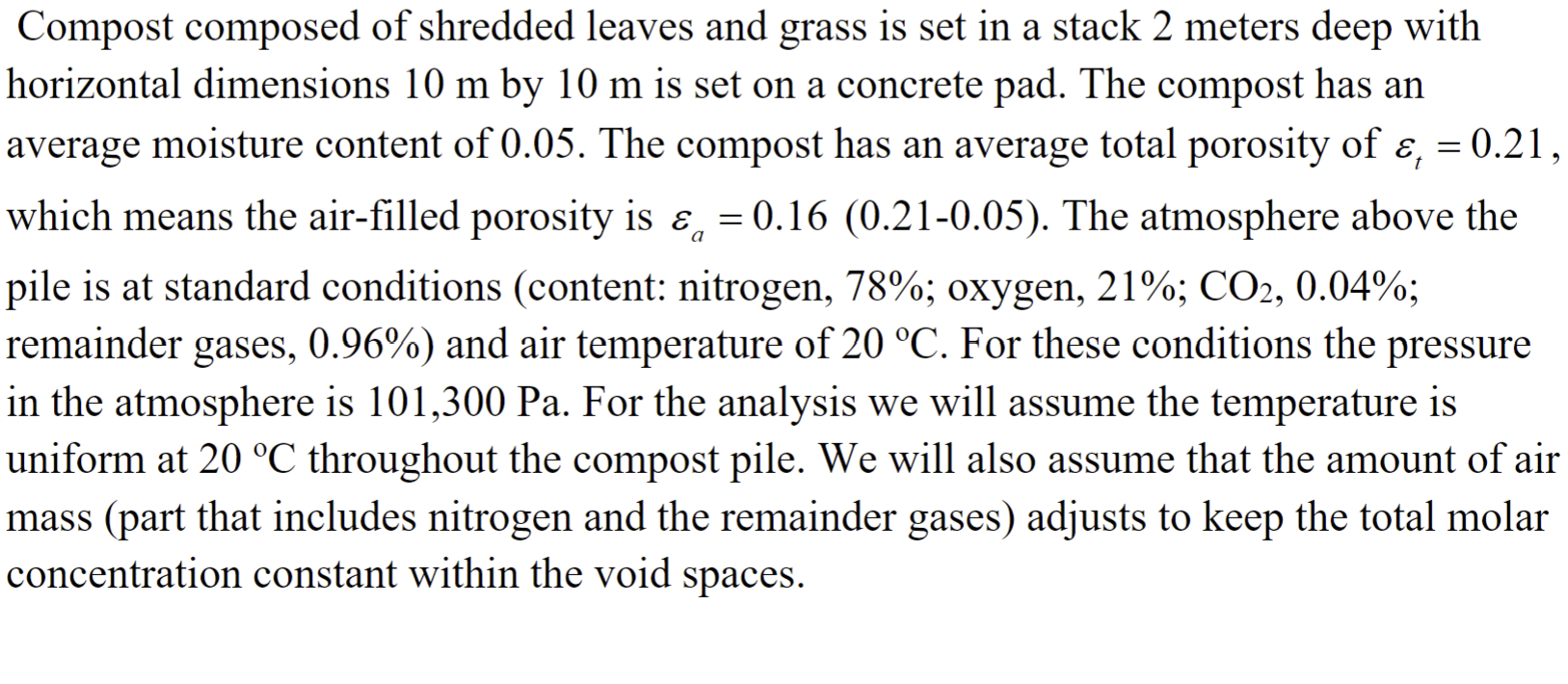
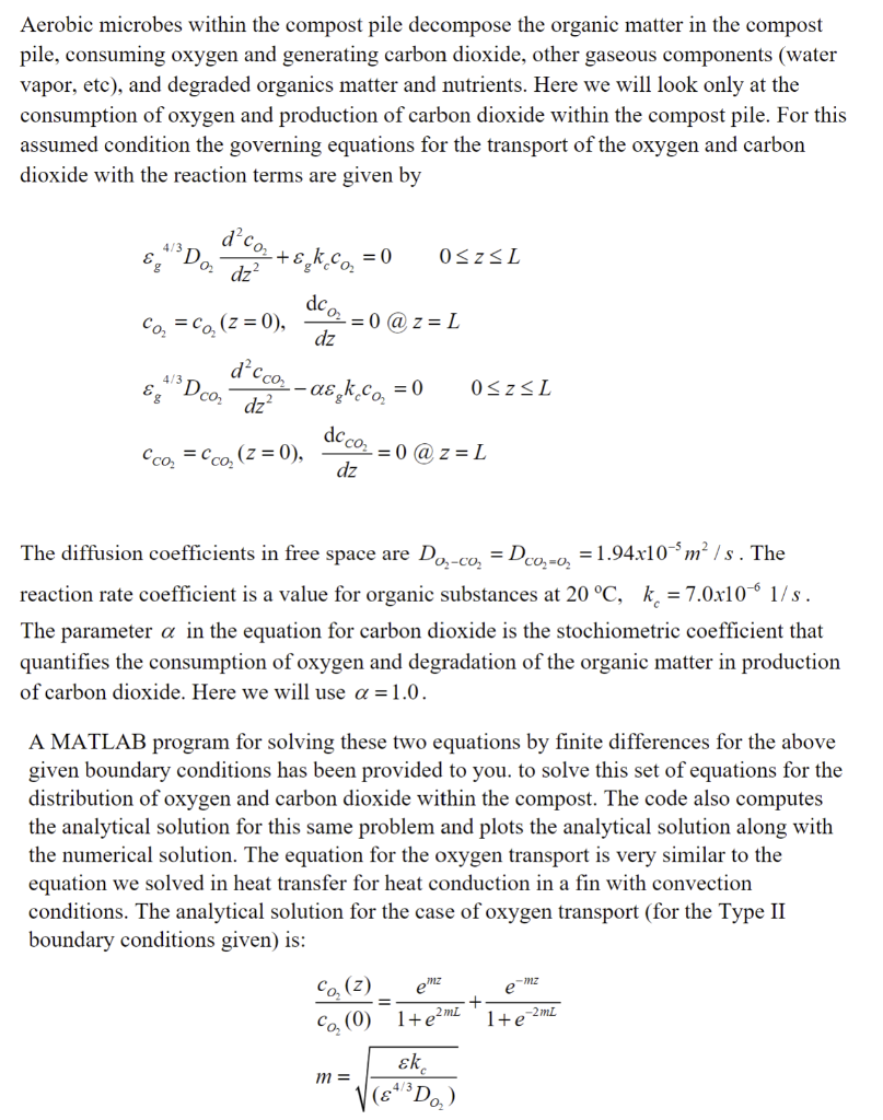
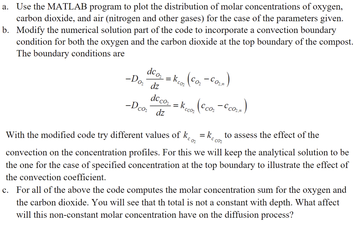
Compost composed of shredded leaves and grass is set in a stack 2 meters deep with horizontal dimensions 10m by 10m is set on a concrete pad. The compost has an average moisture content of 0.05 . The compost has an average total porosity of t=0.21, which means the air-filled porosity is a=0.16(0.210.05). The atmosphere above the pile is at standard conditions (content: nitrogen, 78%; oxygen, 21%; CO2,0.04%; remainder gases, 0.96% ) and air temperature of 20C. For these conditions the pressure in the atmosphere is 101,300Pa. For the analysis we will assume the temperature is uniform at 20C throughout the compost pile. We will also assume that the amount of air mass (part that includes nitrogen and the remainder gases) adjusts to keep the total molar concentration constant within the void spaces. Aerobic microbes within the compost pile decompose the organic matter in the compost pile, consuming oxygen and generating carbon dioxide, other gaseous components (water vapor, etc), and degraded organics matter and nutrients. Here we will look only at the consumption of oxygen and production of carbon dioxide within the compost pile. For this assumed condition the governing equations for the transport of the oxygen and carbon dioxide with the reaction terms are given by g4/3DO2dz2d2cO2+gkccO2=00zLcO2=cO2(z=0),dzdcO2=0@z=Lg4/3DCO2dz2d2cCO2gkccO2=00zLcCO2=cCO2(z=0),dzdcCO2=0@z=L The diffusion coefficients in free space are DO2CO2=DCO2=O2=1.94105m2/s. The reaction rate coefficient is a value for organic substances at 20C,kc=7.01061/s. The parameter in the equation for carbon dioxide is the stochiometric coefficient that quantifies the consumption of oxygen and degradation of the organic matter in production of carbon dioxide. Here we will use =1.0. A MATLAB program for solving these two equations by finite differences for the above given boundary conditions has been provided to you. to solve this set of equations for the distribution of oxygen and carbon dioxide within the compost. The code also computes the analytical solution for this same problem and plots the analytical solution along with the numerical solution. The equation for the oxygen transport is very similar to the equation we solved in heat transfer for heat conduction in a fin with convection conditions. The analytical solution for the case of oxygen transport (for the Type II boundary conditions given) is: cO2(0)cO2(z)=1+e2mLemz+1+e2mLemzm=(4/3DO2)kc a. Use the MATLAB program to plot the distribution of molar concentrations of oxygen, carbon dioxide, and air (nitrogen and other gases) for the case of the parameters given. b. Modify the numerical solution part of the code to incorporate a convection boundary condition for both the oxygen and the carbon dioxide at the top boundary of the compost. The boundary conditions are DO2dzdcO2=kcO2(cO2cO2,)DCO2dzdcCO2=kcCO2(cCO2cCO2,) With the modified code try different values of kcO2=kcCO2 to assess the effect of the convection on the concentration profiles. For this we will keep the analytical solution to be the one for the case of specified concentration at the top boundary to illustrate the effect of the convection coefficient. c. For all of the above the code computes the molar concentration sum for the oxygen and the carbon dioxide. You will see that th total is not a constant with depth. What affect will this non-constant molar concentration have on the diffusion process