Code the function greedy_predicator without using numpy/pandas

Please include explanation of the code & the computational complexity

To see the description of the function: Scroll down the information sheet attached to Part 2- Task A.

Input: A data table data of explanatory variables with m rows and n columns and a list of corresponding target variables y.

Output: A tuple (a,b) where a is the weight vector and b the intercept obtained by the greedy strategy

Information sheet to understand how the function works, refer to Part 2- Task A: Greedy Residual Fitting (you can assume that all the functions from part 1 is completed)

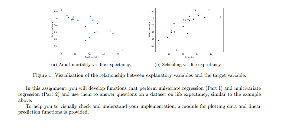
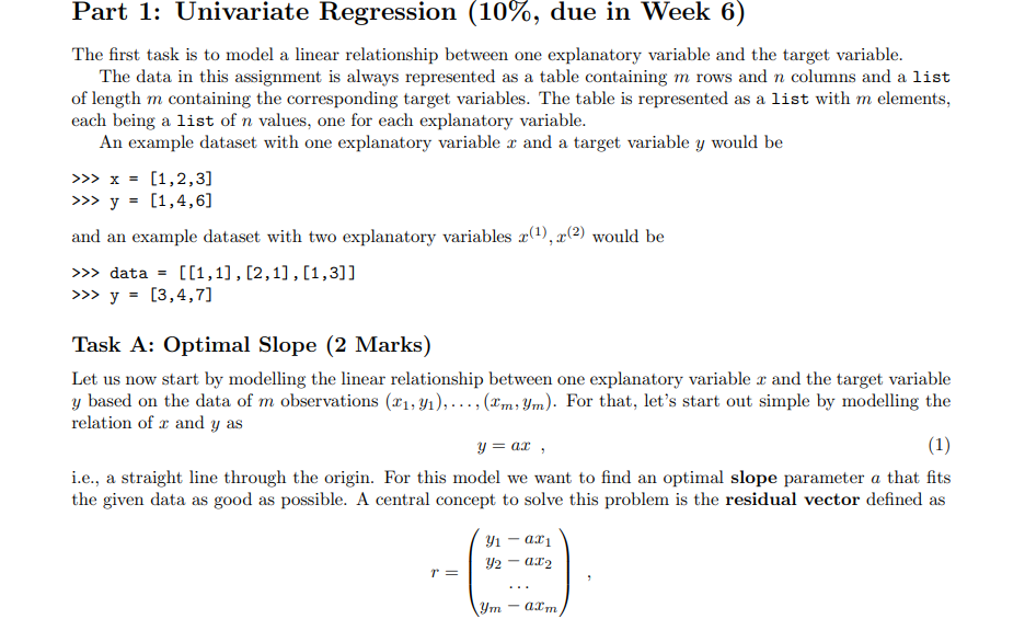
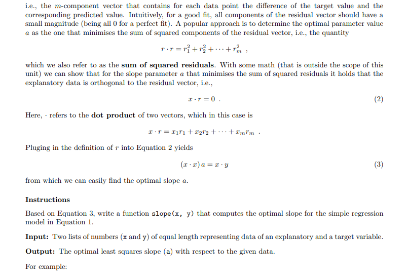
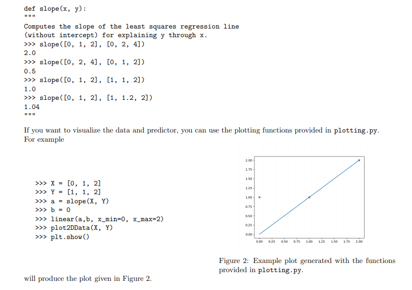
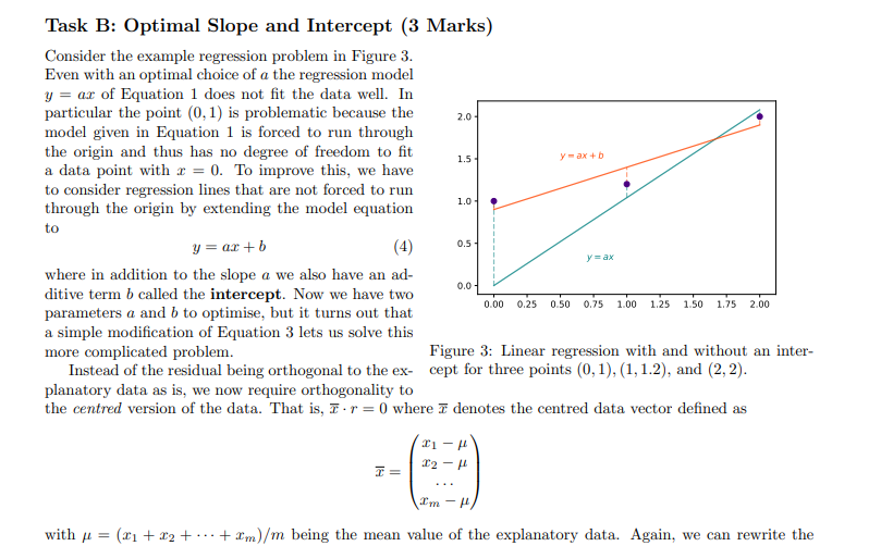
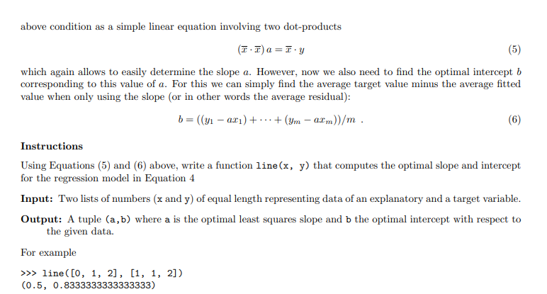
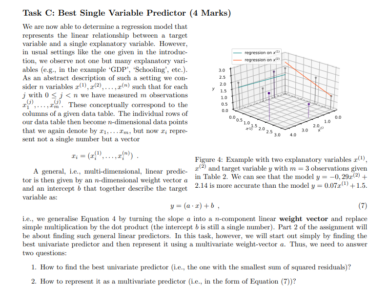
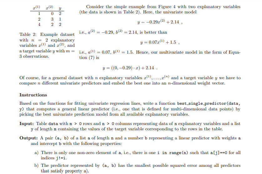
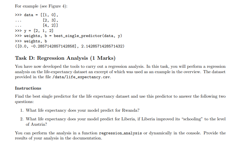
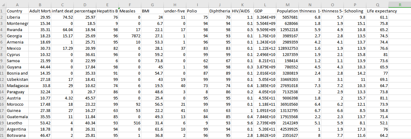
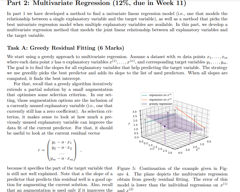
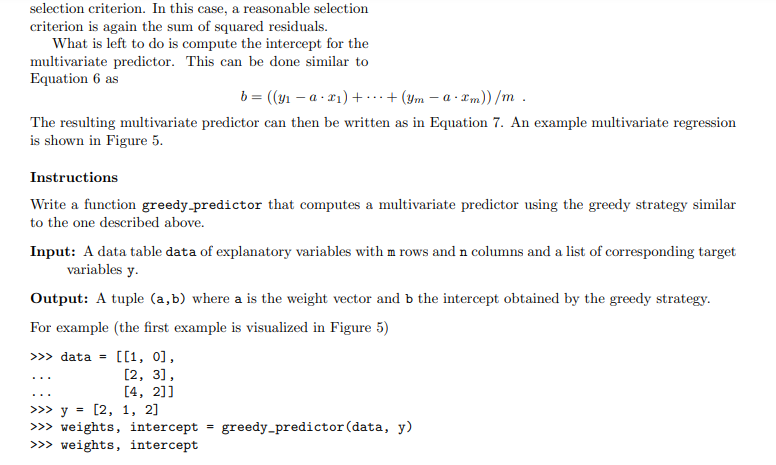
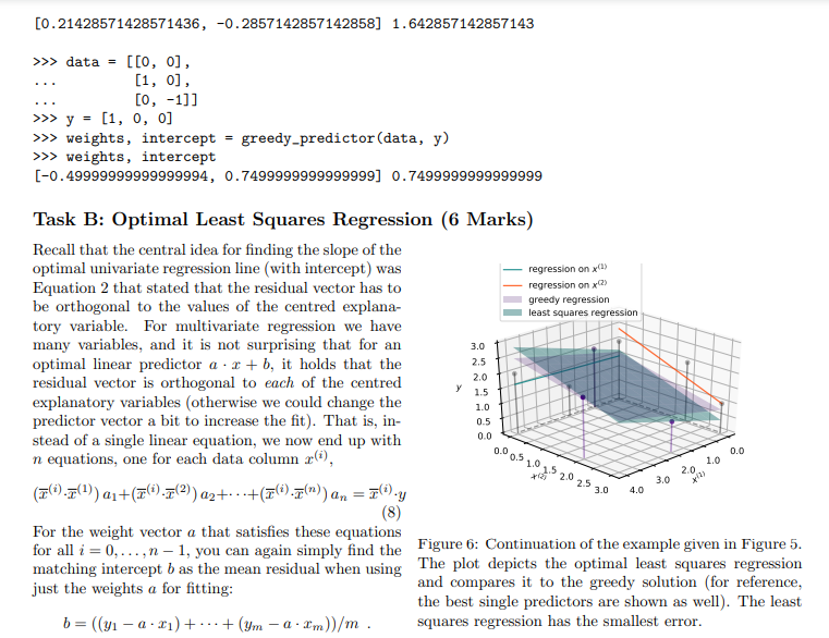
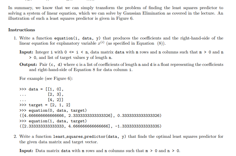
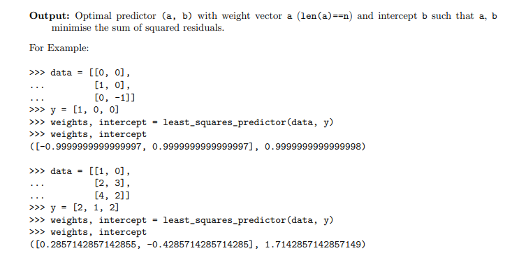
Overview In this assignment we create a Python module to perform some basic data science tasks. While the instructions contain some mathematics, the main focus is on implementing the corresponding algorithms and nding a good decomposition into subproblenis and functions that solve these subpmblems. In particular, we want to implement a method that is able to estimate relationships in observational data and make predictions based on these relationships. For example, consider a dataset that measures the average life expectancy for various countries together with other factors that potentially have an inuence on the life expectancy, such as the average body mass index (BMI), the level of schooling in that country, or the gross domestic product (GDP) {see Table 1 for an example). Can we predict the life expectanCy of Rwanda? And can we predict how the life expectancy of Liberia will change if it improved its schooling to the level of Austria? Country Adult Mortality Infant Deaths BMI GDP Schooling Life expectancy Austria 10.7? 4.32 25.4 4.55e+11 15.7 81.1 Georgia 18.23 15.17 27.1 1.76e+10 13.5 74.5 Liberia 20.05 74.52 24.0 3.264e+00 9.3 61.1 Mexico 30.73 17.2!3.l 28.1 1.22B+12 12.9 75.5 Rwanda 35.31 04.04 22.1 0.509e+09 10.3 ? Table 1: Example dataset on Life Expectancy. To answer these questions, we have to nd the relationships between the target variablein case of this example the life expectancyand the explanatory variablesin this example "Adult Mortality", " Infant Deaths", etc. (see Figure 1}. For this we want to develop a method that nds linear relationships between the explanatory variables and the target variable and use it to understand those relationship and make predictions on the target variable. This method is called a linear regression. The main idea of linear regression is to use data to infer a prediction mction that 'explains' a target variable through linear effects of one or more explanatory variables. Finding the relationship between one particular explanatory variable and the target variable (e.g., the relationship between schooling and life expectanCy} is called a animriote regression. Finding the joint relationship of all explanatory variables with the target variable is called a multivariate regression. TS 75 Life expectancy 65 60 Life expectancy 65 60 - 55 55 10 20 30 40 50 10 12 14 16 Adult Mortality Schooling (a) Adult mortality vs. life expectancy. (b) Schooling vs. life expectancy. Figure 1: Visualization of the relationship between explanatory variables and the target variable. In this assignment, you will develop functions that perform univariate regression (Part I) and multivariate regression (Part 2) and use them to answer questions on a dataset on life expectancy, similar to the example above. To help you to visually check and understand your implementation, a module for plotting data and linear prediction functions is provided.Part 1: Univariate Regression (10%, due in Week 6) The first task is to model a linear relationship between one explanatory variable and the target variable. The data in this assignment is always represented as a table containing m rows and n columns and a list of length m containing the corresponding target variables. The table is represented as a list with m elements, each being a list of n values, one for each explanatory variable. An example dataset with one explanatory variable r and a target variable y would be > >> x = [1,2,3] >>> y = [1,4,6] and an example dataset with two explanatory variables (1), x(2) would be > >> data = [[1, 1] , [2, 1] , [1,3]] >>> y = [3,4,7] Task A: Optimal Slope (2 Marks) Let us now start by modelling the linear relationship between one explanatory variable x and the target variable y based on the data of m observations (X1, y1), . .., (Im, ym). For that, let's start out simple by modelling the relation of r and y as y = at , (1) i.e., a straight line through the origin. For this model we want to find an optimal slope parameter a that fits the given data as good as possible. A central concept to solve this problem is the residual vector defined as y1 - a$1 r = 2 - 012 ym - aimi.e., the m-component vector that contains for each data point the difference of the target value and the corresponding predicted value. Intuitively, for a good fit, all components of the residual vector should have a small magnitude (being all 0 for a perfect fit). A popular approach is to determine the optimal parameter value a as the one that minimises the sum of squared components of the residual vector, i.e., the quantity ror=mitrit . +i'm, which we also refer to as the sum of squared residuals. With some math (that is outside the scope of this unit) we can show that for the slope parameter a that minimises the sum of squared residuals it holds that the explanatory data is orthogonal to the residual vector, i.e., r . r=0 . (2) Here, . refers to the dot product of two vectors, which in this case is Pluging in the definition of r into Equation 2 yields (x . x)a= r . y (3) from which we can easily find the optimal slope a. Instructions Based on Equation 3, write a function slope (x, y) that computes the optimal slope for the simple regression model in Equation 1. Input: Two lists of numbers (x and y) of equal length representing data of an explanatory and a target variable. Output: The optimal least squares slope (a) with respect to the given data. For example:def slope (x, y) : Computes the slope of the least squares regression line (without intercept) for explaining y through x. > >> slope( [0, 1, 2], [0, 2, 4]) 2.0 > >> slope( [0, 2, 4], [0, 1, 2]) 0.5 >>> slope ( [0, 1, 2], [1, 1, 2]) 1.0 > >> slope( [0, 1, 2] , [1, 1.2, 2]) 1. 04 If you want to visualize the data and predictor, you can use the plotting functions provided in plotting. py. For example 2.00 175- >>> X = [0, 1, 2] 150 >>> Y = [1, 1, 2] 125 > >> a = slope (X, Y) 100 > > > b = 0 0.75 > >> linear(a,b, x_min=0, x_max=2) 0.50 >>> plot2DData(X, Y) 0.25 > > > plt . show () 0.00 6.00 025 050 075 1.00 1.25 1.50 175 2.00 Figure 2: Example plot generated with the functions will produce the plot given in Figure 2. provided in plotting. py.Task B: Optimal Slope and Intercept (3 Marks) Consider the example regression problem in Figure 3. Even with an optimal choice of a the regression model y = ar of Equation 1 does not fit the data well. In particular the point (0, 1) is problematic because the 2.0 model given in Equation 1 is forced to run through the origin and thus has no degree of freedom to fit - ax + 6 a data point with x = 0. To improve this, we have 1.5 to consider regression lines that are not forced to run through the origin by extending the model equation 1.0 to y = ar + b (4) 0.5- Y = ax where in addition to the slope a we also have an ad- ditive term b called the intercept. Now we have two 0.0 parameters a and b to optimise, but it turns out that 0.00 0.25 0.50 0.75 1.00 1.25 1.50 1.75 2.00 a simple modification of Equation 3 lets us solve this more complicated problem. Figure 3: Linear regression with and without an inter- Instead of the residual being orthogonal to the ex- cept for three points (0, 1), (1, 1.2), and (2, 2). planatory data as is, we now require orthogonality to the centred version of the data. That is, I . r = 0 where I denotes the centred data vector defined as 12 - 1 I'm with A = (21 + x2+ ..+ I'm)/m being the mean value of the explanatory data. Again, we can rewrite theabove condition as a simple linear equation involving two dot-products (7 . T)a = I . y (5) which again allows to easily determine the slope a. However, now we also need to find the optimal intercept b corresponding to this value of a. For this we can simply find the average target value minus the average fitted value when only using the slope (or in other words the average residual): b = ((y1 - ari) + ...+ (Um - arm))/m . (6) Instructions Using Equations (5) and (6) above, write a function line (x, y) that computes the optimal slope and intercept for the regression model in Equation 4 Input: Two lists of numbers (x and y) of equal length representing data of an explanatory and a target variable. Output: A tuple (a, b) where a is the optimal least squares slope and b the optimal intercept with respect to the given data. For example > >> line( [0, 1, 2] , [1, 1, 2]) (0.5, 0. 8333333333333333)Task C: Best Single Variable Predictor {4 Marks} We are now able to determine a regremion model that represents the linear relationship between a. target variable and a. single explanatory variable. However? in usual settings like the one given in the introduc- mumssionmxm tion, we observe not one but many explanatory vari- newsman-um Q1: ables {e.g., in the example 'GDP', 'Schooling', etc}. so I ' H As an abstract description of such a setting we con- 2-5 I sider n. variables a\"). rig}, . .. ,3\") such that for each I i: I j with I} E j c: n we have measured m observations 1.0 I riy .. ,ri. These conceptually correspond to the '15 columns of a given data table. The individual rows of our data table then become radimensional data points that we again denote by $1,. . .rm, but now 1,- repre- I ' 2.5 3-\" -* sent not a single number but a vector ' _ _ U) (\"l 3' _ {Ii ' \" "m" J' ' Figure 4: Example with two explanatory variables mm, A general i e multi dimensional linear predic- em and target variable y with m = 3 observations given ' ' I? ! tor is then given by an mdimensional weight vector a in Table 2' We can see that the model 3; = _u'(23${2} + and an intercept b that together describe the target 2.141s more accurate than the model 3.- = (l'r +1.5. variable as: y={a-a')+b, (I?) i.e., we generalise Equation 4 by turning the slope a into a n-component linear weight vector and replace simple multiplication by the dot product (the intercept b is still a single number). Part 2 of the assignment will be about nding such general linear predictors. In this task, however. we will start out simply by nding the bait univariate predictor and then represent it using a multivariate weight-vector 0.. Thus? we need to answer two questions: 1. How to nd the best univariate predictor {i.e., the one with the smallest sum of squared residuals}? 2. How to represent it as a multivariate predictor [i.e., in the form of Equation {U}? (2) y Consider the simple example from Figure 4 with two explanatory variables 1:9 05 C (the data is shown in Table 2). Here, the univariate model y = -0.29r(-) + 2.14 , Table 2: Example dataset i.e., a()= -0.29, b(2) = 2.14, is better than with n = 2 explanatory variables x(1) and a(2), and y = 0.07x() +1.5 , a target variable y with m = je., q(1) = 0.07, b(1) = 1.5. Hence, our multivariate model in the form of Equa- 3 observations. tion (7) is y = ((0, -0.29) . x) + 2.14 . Of course, for a general dataset with n explanatory variables r(),...,r(") and a target variable y we have to compare n different univariate predictors and embed the best one into an n-dimensional weight vector. Instructions Based on the functions for fitting univariate regression lines, write a function best_single_predictor (data, y) that computes a general linear predictor (i.e., one that is defined for multi-dimensional data points) by picking the best univariate prediction model from all available explanatory variables. Input: Table data with m > 0 rows and n > 0 columns representing data of n explanatory variables and a list y of length m containing the values of the target variable corresponding to the rows in the table. Output: A pair (a, b) of a list a of length n and a number b representing a linear predictor with weights a and intercept b with the following properties: a) There is only one non-zero element of a, i.e., there is one i in range (n) such that a [j]==0 for all indices j!=i. b) The predictor represented by (a, b) has the smallest possible squared error among all predictors that satisfy property a).For example (see Figure 4): > >> data = [[1, 0], [2, 3] , [4, 2]] )>> y = [ 2, 1, 2] > >> weights, b = best_single_predictor (data, y) > >> weights, b ([0.0, -0. 2857142857142858], 2. 1428571428571432) Task D: Regression Analysis (1 Marks) You have now developed the tools to carry out a regression analysis. In this task, you will perform a regression analysis on the life-expectancy dataset an excerpt of which was used as an example in the overview. The dataset provided in the file /data/life_expectancy . csv. Instructions Find the best single predictor for the life expectancy dataset and use this predictor to answer the following two questions: 1. What life expectancy does your model predict for Rwanda? 2. What life expectancy does your model predict for Liberia, if Liberia improved its "schooling" to the level of Austria? You can perform the analysis in a function regression analysis or dynamically in the console. Provide the results of your analysis in the documentation.B C G H K M R Country Adult Mort infant deat percentage Hepatitis B Measles BMI under-five Polio Diphtheria HIV/AIDS GDP Population thinness 1- thinness 5- Schooling Life expectancy Liberia 29.95 74.52 25.97 76 24 11 75 76 1.1 3.264E+09 5057681 6.8 5.7 9.8 61.1 Montenegr 15.34 18.5 6.7 94 94 0.1 5.504E+09 628066 1.8 1.9 15.1 75.8 Rwanda 35.31 64.04 18.94 98 17 17 98 98 0.5 9.509E+09 12952218 5.9 4.9 10.8 65.2 Georgia 18.23 15.17 25.69 96 7872 1 94 93 0.1 1.76E+10 3989167 2.7 2.8 13.5 74.5 Armenia 18.69 25.71 95 10 53.3 1 96 95 0.1 1.243E+10 2989359 4.2 4.1 74.4 Mexico 30.73 17.29 20.99 82 0 28.1 37 83 83 0.1 1.22E+12 128932753 1.6 1.9 13.9 76.6 Cyprus 10.32 0 36.61 96 59.2 0 99 99 0.1 2.496E+10 1207359 1.9 2.1 15.8 81 21.99 0 22.99 0 62 67 0.1 8.21E+11 198414 1.2 1.1 13.9 73.6 10 Guyana 44.44 0 17.84 98 45 1 98 98 0.3 3.879E+09 786552 4.5 4.3 10.3 65.9 Bosnia and 14.35 0 35.33 91 54.7 O 87 89 0.1 2.016E+10 3280819 2.4 2.8 14.2 77 12 Uzbekistan 27.18 17 99 43 19 99 99 0.1 5.05E+10 33469203 3 3.1 11 3 Madagascar 33.8 29 10.62 74 19.5 40 73 74 0.4 1.385E+10 27691018 7.3 7.2 10.3 64.7 4 Paraguay 32.24 3 20.7 86 48.6 3 8 86 0.2 4.05E+10 7132538 2.9 13.3 73.8 10.77 4.32 45.57 95 0 0 95 95 0.1 4.55E+11 9006398 1.8 15.7 6 Morocco 17.48 18 23.22 99 92 21 99 99 0.1 1.18E+11 36910560 6.4 6.2 73.9 17 Guinea 27.38 27 16.27 63 53 22.2 41 63 63 1 1.091E+10 13132795 6.7 6.6 8.5 58.8 8 Guatemala 35.55 11 11.84 85 49.3 13 84 85 0.4 7.846E+10 17915568 2.2 2.3 13.7 71.4 19 Lesotho 53.42 4 40.34 93 516 31.4 6 9 93 9.6 2.739E+09 2142249 5.1 5.9 8.1 52.1 10 Argentina 18.78 8 26.31 94 61.6 10 99 94 0.1 5.20E+11 42539925 1.9 17.3 76 Botswana 2 25.81 95 1 36.8 2 96 95 2.8 1.862E+10 2351627 8 7.7 11.6 64.2Part 2: Multivariate Regression (12%, due in Week 11) In part 1 we have developed a method to find a univariate linear regression model (i.e., one that models the relationship between a single explanatory variable and the target variable), as well as a method that picks the best univariate regression model when multiple explanatory variables are available. In this part, we develop a multivariate regression method that models the joint linear relationship between all explanatory variables and the target variable. Task A: Greedy Residual Fitting (6 Marks) We start using a greedy approach to multivariate regression. Assume a dataset with m data points $1, ..., I'm where each data point r has n explanatory variables r(), ..., x("), and corresponding target variables y1, . .. ; ym. The goal is to find the slopes for all explanatory variables that help predicting the target variable. The strategy we use greedily picks the best predictor and adds its slope to the list of used predictors. When all slopes are computed, it finds the best intercept. For that, recall that a greedy algorithm iteratively extends a partial solution by a small augmentation that optimises some selection criterion. In our set- regression on x( ting, those augmentation options are the inclusion of regression on x() a currently unused explanatory variable (i.e., one that greedy regression currently still has a zero coefficient). As selection cri- 3.0 terion, it makes sense to look at how much a pre- 2.5 viously unused explanatory variable can improve the 2.0 data fit of the current predictor. For that, it should 1.5 1.0 be useful to look at the current residual vector 0.5 0.0 r = 12 - a - 12 0.0 0.5 1.0 1.5 2.0 2.5 30 2.0 1.0 4.0 3.0 - a . I'm because it specifies the part of the target variable that Figure 5: Continuation of the example given in Fig- is still not well explained. Note that a the slope of a ure 4. The plane depicts the multivariate regression predictor that predicts this residual well is a good op- obtain from greedy residual fitting. The error of this tion for augmenting the current solution. Also, recall model is lower than the individual regressions on r() that an augmentation is used only if it improves the and +(2)selection criterion. In this case, a reasonable selection criterion is again the sum of squared residuals. What is left to do is compute the intercept for the multivariate predictor. This can be done similar to Equation 6 as b = ((m1 -a . ri) + ...+ (ym - a - I'm)) /m . The resulting multivariate predictor can then be written as in Equation 7. An example multivariate regression is shown in Figure 5. Instructions Write a function greedy_predictor that computes a multivariate predictor using the greedy strategy similar to the one described above. Input: A data table data of explanatory variables with m rows and n columns and a list of corresponding target variables y. Output: A tuple (a,b) where a is the weight vector and b the intercept obtained by the greedy strategy. For example (the first example is visualized in Figure 5) >>> data = [[1, 0] , [2, 3] , [4, 2]] >>> y = [2, 1, 2] >>> weights, intercept = greedy_predictor (data, y) > >> weights, intercept[0. 21428571428571436, -0. 2857142857142858] 1. 642857142857143 >>> data = [[0, 0] , [1, 0] , [0, -1]] >>> y = [1, o, 0] >>> weights, intercept = greedy_predictor (data, y) >>> weights, intercept [-0. 49999999999999994, 0. 7499999999999999] 0.7499999999999999 Task B: Optimal Least Squares Regression (6 Marks) Recall that the central idea for finding the slope of the optimal univariate regression line (with intercept) was regression on x(!) Equation 2 that stated that the residual vector has to regression on x(2) be orthogonal to the values of the centred explanat greedy regression least squares regression tory variable. For multivariate regression we have many variables, and it is not surprising that for an 3.0 optimal linear predictor a . r + b, it holds that the 2.5 residual vector is orthogonal to each of the centred 2.0 explanatory variables (otherwise we could change the 1.5 1.0 predictor vector a bit to increase the fit). That is, in- 0.5 stead of a single linear equation, we now end up with 0.0 n equations, one for each data column r(), 0.0 0.5 1.0 1 1.0 12 20 25 30 4.0 3.0 2.0 (7().()) alt (7().(2)) a2+. .+ (7(1).(") ) an = =().y (8) For the weight vector a that satisfies these equations for all i = 0. . ...n - 1, you can again simply find the Figure 6: Continuation of the example given in Figure 5. matching intercept b as the mean residual when using The plot depicts the optimal least squares regression just the weights a for fitting: and compares it to the greedy solution (for reference, the best single predictors are shown as well). The least b = ((31 - a . x1) + ...+ (Um - a . I'm))/m . squares regression has the smallest error.In summary, we know that we can simply transform the problem of finding the least squares predictor to solving a system of linear equation, which we can solve by Gaussian Elimination as covered in the lecture. An illustration of such a least squares predictor is given in Figure 6. Instructions 1. Write a function equation (i, data, y) that produces the coefficients and the right-hand-side of the linear equation for explanatory variable r() (as specified in Equation (8)). Input: Integer i with 0 0 and n > 0, and list of target values y of length n. Output: Pair (c, d) where c is a list of coefficients of length n and d is a float representing the coefficients and right-hand-side of Equation 8 for data column i. For example (see Figure 6): > > > data = [[1, 0] , [2, 3] , [4, 2]] > >> target = [2, 1, 2] >>> equation(0, data, target) ([4 . 666666666666666, 2.3333333333333326], 0.3333333333333326) > >> equation(1, data, target) ([2.333333333333333, 4.666666666666666], -1.3333333333333335) 2. Write a function least_squares_predictor (data, y) that finds the optimal least squares predictor for the given data matrix and target vector. Input: Data matrix data with m rows and n columns such that m > 0 and n > 0.Output: Optimal predictor (a, b) with weight vector a (len(a)==n) and intercept b such that a, b minimise the sum of squared residuals. For Example: >>> data = [[0, 0] , [1, 0] , [0, -1]] >>> y = [, o, 0] > >> weights, intercept = least_squares_predictor (data, y) > >> weights, intercept ([-0. 9999999999999997, 0. 9999999999999997], 0. 9999999999999998) >>> data = [[1, 0] , [2, 3] , [4, 2]] >>> y = [2, 1, 2] > >> weights, intercept = least_squares_predictor (data, y) > >> weights, intercept ([0 . 2857142857142855, -0. 4285714285714285], 1.7142857142857149)