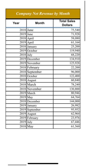
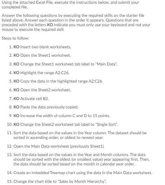
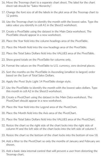Company Net Revenue by Month Year Month 2018 June 2019 June 2018 April 2019 April 2018 January 2019 October 2018 July 2019 December 2019 November 2018 February 2018 September 2018 October 2018 August 2018 March 2018 November 2019 March 2019 May 2018 December 2019 January 2019 September 2019 August 2019 February 2019 July 2018 May Total Sales Dollars 75,540 71,928 58,080 61,164 25,2001 119,940 68.220 134,910 125,928 22,200 96,000 122,400 60,840 78,240 130,800 80,946 64,764 144,000 26,982 95,952 62,964 23,976 67,446 61,5601 Using the attached Excel File, execute the instructions below, and submit your completed file. Answer the following questions by executing the required skills on the starter file listed above. Answer each question in the order it appears. Questions that are preceded with the letters KO indicate you must only use your keyboard and not your mouse to execute the required skill. Steps to follow: 1. KO Insert two blank worksheets. 2. KO Open the Sheet1 worksheet. 3. KO Change the Sheet1 worksheet tab label to "Main Data" 4. KO Highlight the range A2:C26. 5. KO Copy the data in the highlighted range A2:C26. 6. KO Open the Sheet2 worksheet. 7. KO Activate cell B2. 8. KO Paste the data previously copied. 9. KO Increase the width of column C and D to 15 points. 10. Ko Change the Sheet2 worksheet tab label to "Single Sort". 11. Sort the data based on the values in the Year column. The dataset should be sorted in ascending order, or oldest to newest year. 12. Open the Main Data worksheet (previously Sheet1). 13. Sort the data based on the values in the Year and Month columns. The data should be sorted with the oldest (or smallest value) year appearing first. Then, the data should be sorted based on the month in calendar year order. 14. Create an imbedded Treemap chart using the data in the Main Data worksheet. 15. Change the chart title to "Sales by Month Hierarchy". 16. Move the Treemap chart to a separate chart sheet. The label for the chart sheet tab should be "Sales Hierarchy 17. Change the font size of all the labels in the plot area of the treemap chart to 12 points. 18. Use the Treemap chart to identify the month with the lowest sales. Type the sales value you identity in cell A1 in the Sheet3 worksheet 19. Create a PivotTable using the dataset in the Main Data worksheet. The Pivottable should appear in a new worksheet. 20. Place the Year field into the column headings area of the Pivottable. 21. Place the Month field into the row headings area of the Pivot Table 22. Place the Total Sales Dollars field into the VALUES area of the Pivot Table 23. Show grand totals on the Pivottable for columns only. 24. Format the values on the Pivottable to U.S.currency, zero decimal places. 25. Sort the months on the PivotTable in Ascending (smallest to largest) order based on the Sum of Total Sales Dollars. 26. Apply the Pivot Style Light 14 PivotTable design style 27. Use the Pivottable to identify the month with the lowest sales dollars. Type this month in cell A2 in the Sheet3 worksheet. 28. Create a PivotChart using the dataset in the Main Data worksheet. The PivotChart should appear in a new worksheet. 29. Place the Year field into the Legend area of the PivotChart. 30. Place the Month field into the Axis area of the PivotChart. 31. Place the Total Sales Dollars field into the VALUES area of the PivotChart. 32. Resize the chart so the right side of the chart locks into the right side of column M and the left side of the chart locks into the left side of column F. 33. Resize the chart so the bottom of the chart locks into the bottom of row 18. 34. Add a filter to the PivotChart so only the months of January and February are shown. 35. Add a basic data internal control that will prevent a user from distorting the Treemap chart. Company Net Revenue by Month Year Month 2018 June 2019 June 2018 April 2019 April 2018 January 2019 October 2018 July 2019 December 2019 November 2018 February 2018 September 2018 October 2018 August 2018 March 2018 November 2019 March 2019 May 2018 December 2019 January 2019 September 2019 August 2019 February 2019 July 2018 May Total Sales Dollars 75,540 71,928 58,080 61,164 25,2001 119,940 68.220 134,910 125,928 22,200 96,000 122,400 60,840 78,240 130,800 80,946 64,764 144,000 26,982 95,952 62,964 23,976 67,446 61,5601 Using the attached Excel File, execute the instructions below, and submit your completed file. Answer the following questions by executing the required skills on the starter file listed above. Answer each question in the order it appears. Questions that are preceded with the letters KO indicate you must only use your keyboard and not your mouse to execute the required skill. Steps to follow: 1. KO Insert two blank worksheets. 2. KO Open the Sheet1 worksheet. 3. KO Change the Sheet1 worksheet tab label to "Main Data" 4. KO Highlight the range A2:C26. 5. KO Copy the data in the highlighted range A2:C26. 6. KO Open the Sheet2 worksheet. 7. KO Activate cell B2. 8. KO Paste the data previously copied. 9. KO Increase the width of column C and D to 15 points. 10. Ko Change the Sheet2 worksheet tab label to "Single Sort". 11. Sort the data based on the values in the Year column. The dataset should be sorted in ascending order, or oldest to newest year. 12. Open the Main Data worksheet (previously Sheet1). 13. Sort the data based on the values in the Year and Month columns. The data should be sorted with the oldest (or smallest value) year appearing first. Then, the data should be sorted based on the month in calendar year order. 14. Create an imbedded Treemap chart using the data in the Main Data worksheet. 15. Change the chart title to "Sales by Month Hierarchy". 16. Move the Treemap chart to a separate chart sheet. The label for the chart sheet tab should be "Sales Hierarchy 17. Change the font size of all the labels in the plot area of the treemap chart to 12 points. 18. Use the Treemap chart to identify the month with the lowest sales. Type the sales value you identity in cell A1 in the Sheet3 worksheet 19. Create a PivotTable using the dataset in the Main Data worksheet. The Pivottable should appear in a new worksheet. 20. Place the Year field into the column headings area of the Pivottable. 21. Place the Month field into the row headings area of the Pivot Table 22. Place the Total Sales Dollars field into the VALUES area of the Pivot Table 23. Show grand totals on the Pivottable for columns only. 24. Format the values on the Pivottable to U.S.currency, zero decimal places. 25. Sort the months on the PivotTable in Ascending (smallest to largest) order based on the Sum of Total Sales Dollars. 26. Apply the Pivot Style Light 14 PivotTable design style 27. Use the Pivottable to identify the month with the lowest sales dollars. Type this month in cell A2 in the Sheet3 worksheet. 28. Create a PivotChart using the dataset in the Main Data worksheet. The PivotChart should appear in a new worksheet. 29. Place the Year field into the Legend area of the PivotChart. 30. Place the Month field into the Axis area of the PivotChart. 31. Place the Total Sales Dollars field into the VALUES area of the PivotChart. 32. Resize the chart so the right side of the chart locks into the right side of column M and the left side of the chart locks into the left side of column F. 33. Resize the chart so the bottom of the chart locks into the bottom of row 18. 34. Add a filter to the PivotChart so only the months of January and February are shown. 35. Add a basic data internal control that will prevent a user from distorting the Treemap chart