Complete the Pivot Table in Excel:

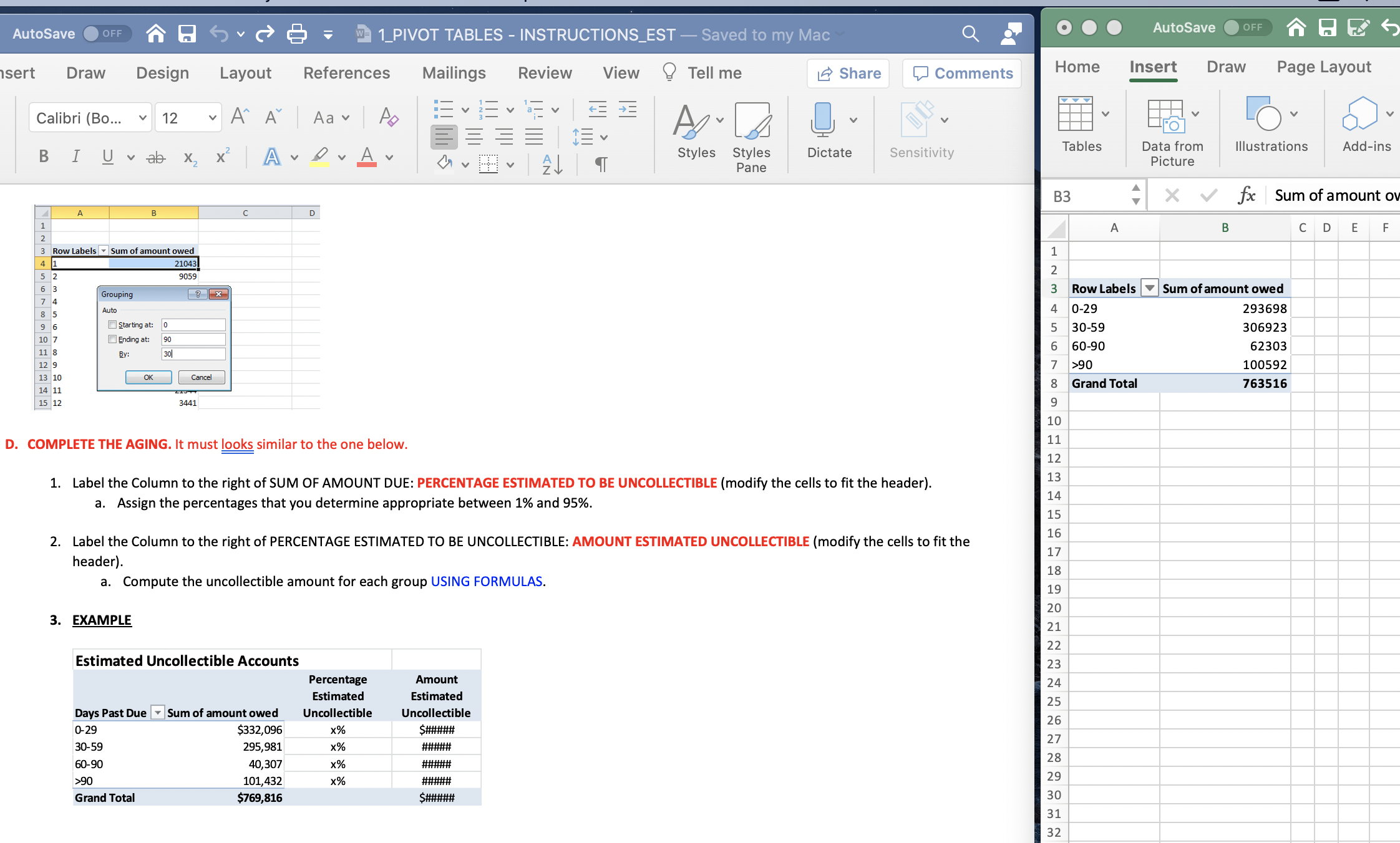
AutoSave OFF AutoSave OFF Sv 1_PIVOT TABLES - INSTRUCTIONS_EST - Saved to my Mac nsert Draw References Design Layout Review Home View Mailings Insert Tell me Draw Share o Comments Page Layout Calibri (Bo... V V 12 V po Ai k Aav vab x, x Ave A Tables == AL Add-ins B Illustrations I U Dictate Sensitivity Data from Picture Styles Styles Pane 90 90 6 By: 30 7 11 8 12 9 13 10 14 11 OK Cancel 8 Grand Total 15 12 3441 9 10 11 D. COMPLETE THE AGING. It must looks similar to the one below. 1. Label the Column to the right of SUM OF AMOUNT DUE: PERCENTAGE ESTIMATED TO BE UNCOLLECTIBLE (modify the cells to fit the header). a. Assign the percentages that you determine appropriate between 1% and 95%. 12 13 14 15 16 17 2. Label the Column to the right of PERCENTAGE ESTIMATED TO BE UNCOLLECTIBLE: AMOUNT ESTIMATED UNCOLLECTIBLE (modify the cells to fit the header). a. Compute the uncollectible amount for each group USING FORMULAS. 18 19 20 3. EXAMPLE 21 22 23 24 25 Estimated Uncollectible Accounts Percentage Estimated Days Past Due Sum of amount owed Uncollectible 0-29 $332,096 x% 30-59 295,981 x% 60-90 40,307 x% >90 101,432 x% Grand Total $769,816 Amount Estimated Uncollectible $##### ##### 26 27 28 ##### 29 ##### $##### 30 31 32