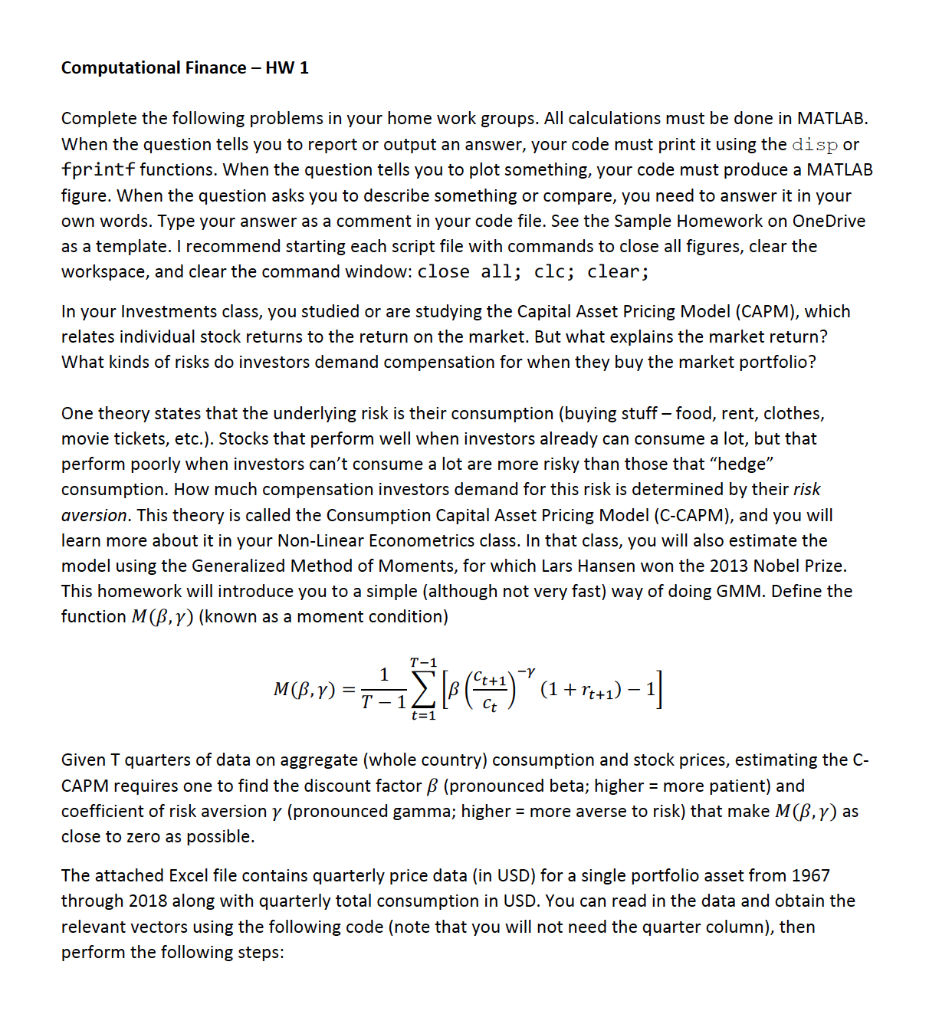
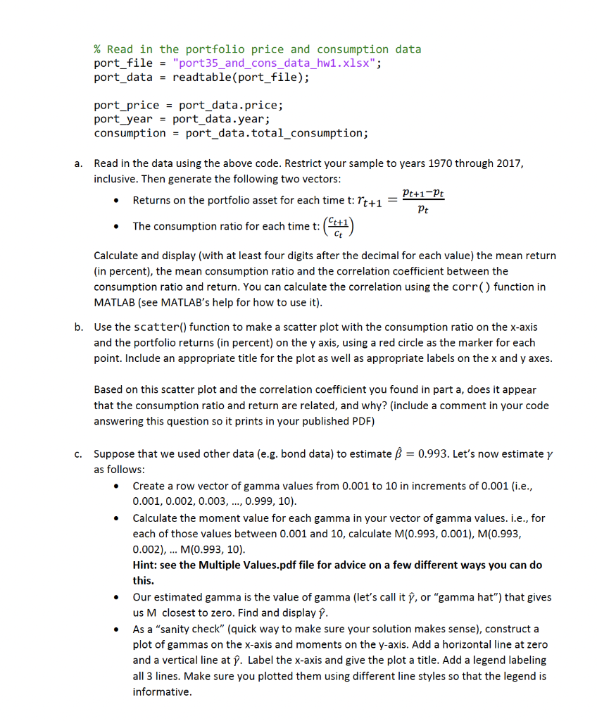
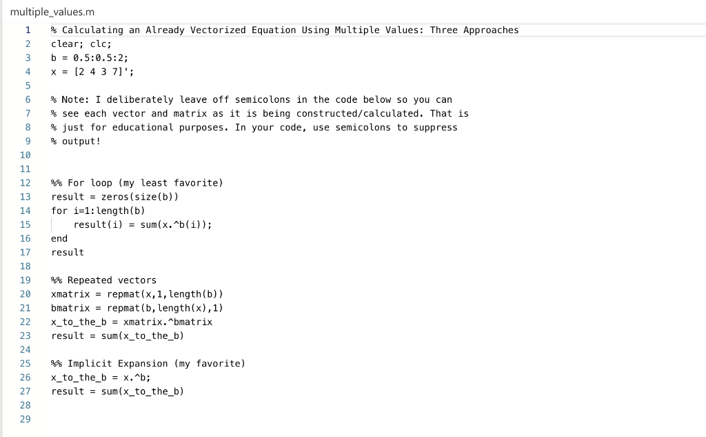
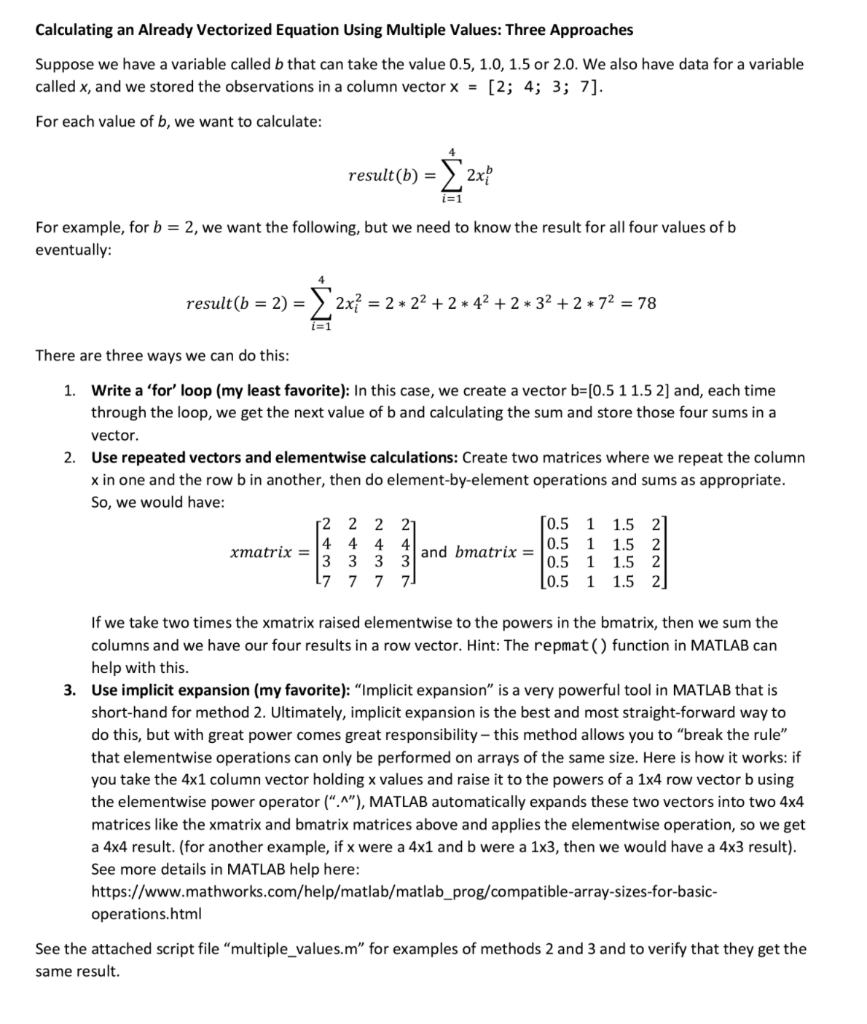
Computational Finance - HW 1 Complete the following problems in your home work groups. All calculations must be done in MATLAB. When the question tells you to report or output an answer, your code must print it using the disp or fprintf functions. When the question tells you to plot something, your code must produce a MATLAB figure. When the question asks you to describe something or compare, you need to answer it in your own words. Type your answer as a comment in your code file. See the Sample Homework on OneDrive as a template. I recommend starting each script file with commands to close all figures, clear the workspace, and clear the command window: close all; clc; clear; In your Investments class, you studied or are studying the Capital Asset Pricing Model (CAPM), which relates individual stock returns to the return on the market. But what explains the market return? What kinds of risks do investors demand compensation for when they buy the market portfolio? One theory states that the underlying risk is their consumption (buying stuff - food, rent, clothes, movie tickets, etc.). Stocks that perform well when investors already can consume a lot, but that perform poorly when investors can't consume a lot are more risky than those that "hedge" consumption. How much compensation investors demand for this risk is determined by their risk aversion. This theory is called the Consumption Capital Asset Pricing Model (C-CAPM), and you will learn more about it in your Non-Linear Econometrics class. In that class, you will also estimate the model using the Generalized Method of Moments, for which Lars Hansen won the 2013 Nobel Prize. This homework will introduce you to a simple (although not very fast) way of doing GMM. Define the function M(B,y) (known as a moment condition) T-1 MB,y) = T-1 t=1 (PC)*(1 + resu) 1] Given T quarters of data on aggregate (whole country) consumption and stock prices, estimating the C- CAPM requires one to find the discount factor B (pronounced beta; higher = more patient) and coefficient of risk aversion y (pronounced gamma; higher = more averse to risk) that make MB,y) as close to zero as possible. The attached Excel file contains quarterly price data (in USD) for a single portfolio asset from 1967 through 2018 along with quarterly total consumption in USD. You can read in the data and obtain the relevant vectors using the following code (note that you will not need the quarter column), then perform the following steps: % Read in the portfolio price and consumption data port_file = "port35_and_cons_data_hw1.xlsx"; port_data = readtable (port_file); port_price = port_data.price; port_year = port_data.year; consumption = port_data.total_consumption; a. Read in the data using the above code. Restrict your sample to years 1970 through 2017, inclusive. Then generate the following two vectors: Returns on the portfolio asset for each time t: rt+1 Pt+1-Pt Pt The consumption ratio for each time t: . . t:(+2) Calculate and display (with at least four digits after the decimal for each value) the mean return (in percent), the mean consumption ratio and the correlation coefficient between the consumption ratio and return. You can calculate the correlation using the corr() function in MATLAB (see MATLAB's help for how to use it). b. Use the scatter() function to make a scatter plot with the consumption ratio on the x-axis and the portfolio returns (in percent) on the y axis, using a red circle as the marker for each point. Include an appropriate title for the plot as well as appropriate labels on the x and y axes. Based on this scatter plot and the correlation coefficient you found in part a, does it appear that the consumption ratio and return are related, and why? (include a comment in your code answering this question so it prints in your published PDF) C. Suppose that we used other data (e.g. bond data) to estimate = 0.993. Let's now estimate y as follows: Create a row vector of gamma values from 0.001 to 10 in increments of 0.001 (i.e., 0.001, 0.002, 0.003, ..., 0.999, 10). Calculate the moment value for each gamma in your vector of gamma values. i.e., for each of those values between 0.001 and 10, calculate M(0.993, 0.001), M(0.993, 0.002),... M(0.993, 10). Hint: see the Multiple Values.pdf file for advice on a few different ways you can do this. Our estimated gamma is the value of gamma (let's call it , or "gamma hat") that gives us M closest to zero. Find and display As a "sanity check" (quick way to make sure your solution makes sense), construct a plot of gammas on the x-axis and moments on the y-axis. Add a horizontal line at zero and a vertical line at y. Label the x-axis and give the plot a title. Add a legend labeling all 3 lines. Make sure you plotted them using different line styles so that the legend is informative. . multiple_values.m 1 % Calculating an Already Vectorized Equation Using Multiple Values: Three Approaches 2 clear; clc; 3 b = 0.5:0.5:2; 4. x = [2 4 3 7]'; 5 6 % Note: I deliberately leave off semicolons in the code below so you can 7 % see each vector and matrix as it is being constructed/calculated. That is 8 % just for educational purposes. In your code, use semicolons to suppress 9 $output! 10 11 12 %% For loop (my least favorite) 13 result = zeros(size(b)) 14 for i=1: length(b) 15 result(i) = Sum(x.ab(i)); 16 end 17 result 18 19 %% Repeated vectors 20 xmatrix = repmat(x,1, length(b)) 21 bmatrix = repmat(b, length(x),1) 22 X_to_the_b = xmatrix.bmatrix 23 result = sum(x_to_the_b) 24 25 $% Implicit Expansion (my favorite) 26 X_to_the_b = x. b; 27 result = sum(x_to_the_b) 28 29 Calculating an Already Vectorized Equation Using Multiple Values: Three Approaches Suppose we have a variable called b that can take the value 0.5, 1.0, 1.5 or 2.0. We also have data for a variable called x, and we stored the observations in a column vector x = [2; 4; 3; 7]. For each value of b, we want to calculate: result(b) = Z 2x = i=1 For example, for b = 2, we want the following, but we need to know the result for all four values of b eventually: result(b = 2) = 2x} = 2 * 22 + 2 * 42 + 2 * 32 + 2 * 72 = 78 i=1 There are three ways we can do this: 1. Write a 'for' loop (my least favorite): In this case, we create a vector b=[0.5 1 1.5 2] and, each time through the loop, we get the next value of b and calculating the sum and store those four sums in a vector. 2. Use repeated vectors and elementwise calculations: Create two matrices where we repeat the column x in one and the row b in another, then do element-by-element operations and sums as appropriate. So, we would have: 12 2 2 2 0.5 1 1.5 2 4 4 4 4 xmatrix = 0.5 1 and bmatrix = 1.5 2 | 3 3 3 3 0.5 1 1.5 2 17 7 7 7 [0.5 1 1.5 2] If we take two times the xmatrix raised elementwise to the powers in the bmatrix, then we sum the columns and we have our four results in a row vector. Hint: The repmat() function in MATLAB can help with this. 3. Use implicit expansion (my favorite): "Implicit expansion" is a very powerful tool in MATLAB that is short-hand for method 2. Ultimately, implicit expansion is the best and most straight-forward way to do this, but with great power comes great responsibility - this method allows you to "break the rule" that elementwise operations can only be performed on arrays of the same size. Here is how it works: if you take the 4x1 column vector holding x values and raise it to the powers of a 1x4 row vector b using the elementwise power operator (.), MATLAB automatically expands these two vectors into two 4x4 matrices like the xmatrix and bmatrix matrices above and applies the elementwise operation, so we get a 4x4 result. (for another example, if x were a 4x1 and b were a 1x3, then we would have a 4x3 result). See more details in MATLAB help here: https://www.mathworks.com/help/matlab/matlab_prog/compatible-array-sizes-for-basic- operations.html See the attached script file "multiple_values.m" for examples of methods 2 and 3 and to verify that they get the same result. 16 17 1970 1970 1971 18 19 15032 15090 15134 15204 15243 20 1971 1971 1971 1972 21 15390 15544 22 23 24 25 1972 1972 1972 1973 1973 26 27 15770 15943 16190 16326 16339 16397 16377 16253 1973 28 29 1973 1974 30 31 32 1974 1974 33 34 35 16297 16326 16309 16391 16598 16652 16763 16965 17086 17226 36 37 38 3 137.6262515 4 148.7194778 1 165.1818317 2 165.3688175 3 167.4129415 4 173.8415984 1 190.745434 2 176.5240266 3 177.8278331 4 190.8702599 1 181.0723168 2 162.4850624 3 187.3457644 4 183.6233914 1 190.4756655 2 167.2471581 3 137.2607461 4 133.0974905 1 171.5010411 2 201.4019046 3 177.9919542 4 199.101444 1 264.7971555 2 274.4603981 3 280.0832683 4 298.1763674 1 300.8238753 2 316.9203592 3 288.8088895 4 295.5003027 1 296.4145806 2 324.1406077 3 352.9336937 4 311.622099 1 353.4286966 2 354.4942841 3 386.8631572 4 377.3002868 1 358.2383217 2 401.2774319 3 419.0789013 39 40 41 17399 17503 42 1974 1975 1975 1975 1975 1976 1976 1976 1976 1977 1977 1977 1977 1978 1978 1978 1978 1979 1979 1979 1979 1980 1980 43 44 45 46 47 48 49 50 51 17506 17613 17793 17968 18152 18232 18316 18428 18449 18505 18585 18552 18344 18425 52 53 54 55 56 1980 B 54 18552 18344 55 56 1980 1980 1980 1980 1981 57 58 59 1981 1981 18425 18594 18529 18600 18564 18563 18603 18626 60 61 62 1981 1982 1982 63 64 18704 1982 1982 66 67 68 69 70 71 56 85 8 9 72 1983 1983 1983 1983 1984 1984 1984 1984 1985 1985 1985 1985 1986 1986 1986 73 74 1 358.2383217 2 401.2774319 3 419.0789013 4 420.1249223 1 477.757239 2 482.7799008 3 471.9598377 4 497.2342309 1 505.2859448 2 494.3182081 3 545.8400063 4649.3607468 1 719.1670271 2 797.758319 3 839.1101215 4 843.8603239 1 891.6084726 2 860.5127355 3 968.45029 4 981.1941273 1 1073.316482 2 1180.307888 3 1130.948593 4 1280.792496 1 1449.763607 2 1524.13793 3 1555.618999 4 1615.104314 1 1885.203054 2 1970.670619 3 2033.842437 4 1659.619496 1 1858.571362 2 1999.939875 3 2023.977153 4 2122.457809 1 2255.746037 2 2456.951816 3 2640.623706 4 2695.00207 1 2642.94002 18918 19076 19286 19524 19690 19729 19923 20056 20209 20467 20603 20796 20916 21012 21111 75 76 77 78 79 80 81 1986 82 83 84 85 1987 1987 1987 1987 1988 1988 1988 1988 86 87 21197 21361 21576 21730 21821 21928 22166 22309 22536 22681 22776 22800 22907 23073 88 89 90 91 92 1989 1989 93 1989 1989 1990 94 23099 A B C D E F 23115 23033 23163 23164 23133 23434 23515 23648 23822 23825 4 2353.397291 1 2662.504258 2 2751.069799 3 2765.595448 4 2823.515313 1 3229.203641 2 3409.829146 3 3266.578814 4 3476.757028 1 3991.501336 24253.415671 3 4249.55357 4 4342.623042 1 4078.491681 2 4008.463979 3 4309.708064 4 4290.13337 1 4609.010403 2 4994.203838 3 5383.661842 4 5708.016701 1 5694.460161 2 5844.076407 3 5730.771454 4 6060.932659 23891 24075 24157 24323 24430 97 1990 98 1991 99 1991 100 1991 101 1991 102 1992 103 1992 104 1992 105 1992 106 1993 107 1993 108 1993 109 1993 110 1994 111 1994 112 1994 113 1994 114 1995 115 1995 116 1995 117 1995 118 1996 119 1996 120 1996 121 1996 122 1997 123 1997 124 1997 125 1997 126 1998 127 1998 128 1998 129 1998 130 1999 131 1999 132 1999 133 1999 134 2000 135 2000 136 2000 137 2000 24525 24626 24708 24851 24927 24986 25149 25268 25334 25412 25550 25622 25869 26044 1 6020.209252 26248 2 6582.563019 3 7139.566337 4 7652.929714 1 8526.779494 2 8427.016174 3 8415.353183 4 9090.937737 1 8604.390749 2 9441.606574 26509 26710 26834 27058 27240 3 8962.322299 27406 4 9540.087368 1 9772.970441 2 9923.19077 3 10978.4328 4 11717.11665 27737 27920 28246 28415 28589 137 2000 28589 28582 28595 28584 28647 28738 28815 28850 29012 29102 29217 29444 29539 29707 29843 30033 30248 30367 138 2001 139 2001 140 2001 141 2001 142 2002 143 2002 144 2002 145 2002 146 2003 147 2003 148 2003 149 2003 150 2004 151 2004 152 2004 153 2004 154 2005 155 2005 156 2005 157 2005 158 2006 159 2006 160 2006 161 2006 162 2007 163 2007 164 2007 165 2007 166 2008 167 2008 168 2008 169 2008 170 2009 171 2009 172 2009 173 2009 174 2010 175 2010 176 2010 177 2010 4 11717.11665 1 11796.17204 2 12217.07125 3 10907.42565 4 11541.038 1 10355.62337 2 7647.731412 3 6470.309627 4 7195.948382 1 6354.792387 2 7851.225254 3 7995.075403 4 9243.89019 1 9634.268917 2 10031.03701 3 10197.16102 4 11571.18768 1 12020.1729 2 12366.93085 3 13433.28183 4 12751.78457 1 13494.372 2 14084.30546 3 14457.48321 4 15958.93622 1 16346.72241 2 17237.01395 3 17031.0144 4 16538.23903 1 15374.98891 2 16060.40592 3 14862.01055 4 11172.75422 1 9881.228524 2 11680.19511 3 14824.72555 4 15620.33893 1 17326.61103 2 14211.26904 3 15488.09472 4 16716.53295 30577 30749 30914 31067 31174 31246 31449 31519 31467 31535 31525 31501 31520 31313 31192 31044 30865 30862 30824 30890 30998 31122 31190 B 30862 30824 30890 30998 31122 31190 31256 31306 31350 31269 31410 31404 31354 31369 31412 31372 A 172 2009 173 2009 174 2010 175 2010 176 2010 177 2010 178 2011 179 2011 180 2011 181 2011 182 2012 183 2012 184 2012 185 2012 186 2013 187 2013 188 2013 189 2013 190 2014 191 2014 192 2014 193 2014 194 2015 195 2015 196 2015 197 2015 198 2016 199 2016 200 2016 201 2016 202 2017 203 2017 204 2017 205 2017 206 2018 207 2018 208 2018 209 2018 210 3 14824.72555 4 15620.33893 1 17326.61103 2 14211.26904 3 15488.09472 4 16716.53295 1 18394.85614 2 18344.32547 3 16272.84755 4 17989.69806 1 19136.68523 2 19613.30351 3 20937.69183 4 21183.68877 1 24379.39651 2 24902.04201 3 25904.02547 4 27807.45326 1 29668.13339 2 31927.24307 3 31152.68815 4 31769.82291 1 30788.13538 2 28996.32747 3 26312.63038 4 27129.00605 1 29841.60823 2 31521.69078 3 31932.89123 4 34094.52444 1 34876.31189 2 34533.44286 3 36606.41637 4 37877.72061 1 37010.85109 2 37419.93203 3 39675.38101 4 35076.25052 31423 31624 31652 31854 32104 32402 32589 32742 32909 32985 33164 33312 33382 33492 33635 33743 33832 34093 34180 34431 34667 34736 Computational Finance - HW 1 Complete the following problems in your home work groups. All calculations must be done in MATLAB. When the question tells you to report or output an answer, your code must print it using the disp or fprintf functions. When the question tells you to plot something, your code must produce a MATLAB figure. When the question asks you to describe something or compare, you need to answer it in your own words. Type your answer as a comment in your code file. See the Sample Homework on OneDrive as a template. I recommend starting each script file with commands to close all figures, clear the workspace, and clear the command window: close all; clc; clear; In your Investments class, you studied or are studying the Capital Asset Pricing Model (CAPM), which relates individual stock returns to the return on the market. But what explains the market return? What kinds of risks do investors demand compensation for when they buy the market portfolio? One theory states that the underlying risk is their consumption (buying stuff - food, rent, clothes, movie tickets, etc.). Stocks that perform well when investors already can consume a lot, but that perform poorly when investors can't consume a lot are more risky than those that "hedge" consumption. How much compensation investors demand for this risk is determined by their risk aversion. This theory is called the Consumption Capital Asset Pricing Model (C-CAPM), and you will learn more about it in your Non-Linear Econometrics class. In that class, you will also estimate the model using the Generalized Method of Moments, for which Lars Hansen won the 2013 Nobel Prize. This homework will introduce you to a simple (although not very fast) way of doing GMM. Define the function M(B,y) (known as a moment condition) T-1 MB,y) = T-1 t=1 (PC)*(1 + resu) 1] Given T quarters of data on aggregate (whole country) consumption and stock prices, estimating the C- CAPM requires one to find the discount factor B (pronounced beta; higher = more patient) and coefficient of risk aversion y (pronounced gamma; higher = more averse to risk) that make MB,y) as close to zero as possible. The attached Excel file contains quarterly price data (in USD) for a single portfolio asset from 1967 through 2018 along with quarterly total consumption in USD. You can read in the data and obtain the relevant vectors using the following code (note that you will not need the quarter column), then perform the following steps: % Read in the portfolio price and consumption data port_file = "port35_and_cons_data_hw1.xlsx"; port_data = readtable (port_file); port_price = port_data.price; port_year = port_data.year; consumption = port_data.total_consumption; a. Read in the data using the above code. Restrict your sample to years 1970 through 2017, inclusive. Then generate the following two vectors: Returns on the portfolio asset for each time t: rt+1 Pt+1-Pt Pt The consumption ratio for each time t: . . t:(+2) Calculate and display (with at least four digits after the decimal for each value) the mean return (in percent), the mean consumption ratio and the correlation coefficient between the consumption ratio and return. You can calculate the correlation using the corr() function in MATLAB (see MATLAB's help for how to use it). b. Use the scatter() function to make a scatter plot with the consumption ratio on the x-axis and the portfolio returns (in percent) on the y axis, using a red circle as the marker for each point. Include an appropriate title for the plot as well as appropriate labels on the x and y axes. Based on this scatter plot and the correlation coefficient you found in part a, does it appear that the consumption ratio and return are related, and why? (include a comment in your code answering this question so it prints in your published PDF) C. Suppose that we used other data (e.g. bond data) to estimate = 0.993. Let's now estimate y as follows: Create a row vector of gamma values from 0.001 to 10 in increments of 0.001 (i.e., 0.001, 0.002, 0.003, ..., 0.999, 10). Calculate the moment value for each gamma in your vector of gamma values. i.e., for each of those values between 0.001 and 10, calculate M(0.993, 0.001), M(0.993, 0.002),... M(0.993, 10). Hint: see the Multiple Values.pdf file for advice on a few different ways you can do this. Our estimated gamma is the value of gamma (let's call it , or "gamma hat") that gives us M closest to zero. Find and display As a "sanity check" (quick way to make sure your solution makes sense), construct a plot of gammas on the x-axis and moments on the y-axis. Add a horizontal line at zero and a vertical line at y. Label the x-axis and give the plot a title. Add a legend labeling all 3 lines. Make sure you plotted them using different line styles so that the legend is informative. . multiple_values.m 1 % Calculating an Already Vectorized Equation Using Multiple Values: Three Approaches 2 clear; clc; 3 b = 0.5:0.5:2; 4. x = [2 4 3 7]'; 5 6 % Note: I deliberately leave off semicolons in the code below so you can 7 % see each vector and matrix as it is being constructed/calculated. That is 8 % just for educational purposes. In your code, use semicolons to suppress 9 $output! 10 11 12 %% For loop (my least favorite) 13 result = zeros(size(b)) 14 for i=1: length(b) 15 result(i) = Sum(x.ab(i)); 16 end 17 result 18 19 %% Repeated vectors 20 xmatrix = repmat(x,1, length(b)) 21 bmatrix = repmat(b, length(x),1) 22 X_to_the_b = xmatrix.bmatrix 23 result = sum(x_to_the_b) 24 25 $% Implicit Expansion (my favorite) 26 X_to_the_b = x. b; 27 result = sum(x_to_the_b) 28 29 Calculating an Already Vectorized Equation Using Multiple Values: Three Approaches Suppose we have a variable called b that can take the value 0.5, 1.0, 1.5 or 2.0. We also have data for a variable called x, and we stored the observations in a column vector x = [2; 4; 3; 7]. For each value of b, we want to calculate: result(b) = Z 2x = i=1 For example, for b = 2, we want the following, but we need to know the result for all four values of b eventually: result(b = 2) = 2x} = 2 * 22 + 2 * 42 + 2 * 32 + 2 * 72 = 78 i=1 There are three ways we can do this: 1. Write a 'for' loop (my least favorite): In this case, we create a vector b=[0.5 1 1.5 2] and, each time through the loop, we get the next value of b and calculating the sum and store those four sums in a vector. 2. Use repeated vectors and elementwise calculations: Create two matrices where we repeat the column x in one and the row b in another, then do element-by-element operations and sums as appropriate. So, we would have: 12 2 2 2 0.5 1 1.5 2 4 4 4 4 xmatrix = 0.5 1 and bmatrix = 1.5 2 | 3 3 3 3 0.5 1 1.5 2 17 7 7 7 [0.5 1 1.5 2] If we take two times the xmatrix raised elementwise to the powers in the bmatrix, then we sum the columns and we have our four results in a row vector. Hint: The repmat() function in MATLAB can help with this. 3. Use implicit expansion (my favorite): "Implicit expansion" is a very powerful tool in MATLAB that is short-hand for method 2. Ultimately, implicit expansion is the best and most straight-forward way to do this, but with great power comes great responsibility - this method allows you to "break the rule" that elementwise operations can only be performed on arrays of the same size. Here is how it works: if you take the 4x1 column vector holding x values and raise it to the powers of a 1x4 row vector b using the elementwise power operator (.), MATLAB automatically expands these two vectors into two 4x4 matrices like the xmatrix and bmatrix matrices above and applies the elementwise operation, so we get a 4x4 result. (for another example, if x were a 4x1 and b were a 1x3, then we would have a 4x3 result). See more details in MATLAB help here: https://www.mathworks.com/help/matlab/matlab_prog/compatible-array-sizes-for-basic- operations.html See the attached script file "multiple_values.m" for examples of methods 2 and 3 and to verify that they get the same result. 16 17 1970 1970 1971 18 19 15032 15090 15134 15204 15243 20 1971 1971 1971 1972 21 15390 15544 22 23 24 25 1972 1972 1972 1973 1973 26 27 15770 15943 16190 16326 16339 16397 16377 16253 1973 28 29 1973 1974 30 31 32 1974 1974 33 34 35 16297 16326 16309 16391 16598 16652 16763 16965 17086 17226 36 37 38 3 137.6262515 4 148.7194778 1 165.1818317 2 165.3688175 3 167.4129415 4 173.8415984 1 190.745434 2 176.5240266 3 177.8278331 4 190.8702599 1 181.0723168 2 162.4850624 3 187.3457644 4 183.6233914 1 190.4756655 2 167.2471581 3 137.2607461 4 133.0974905 1 171.5010411 2 201.4019046 3 177.9919542 4 199.101444 1 264.7971555 2 274.4603981 3 280.0832683 4 298.1763674 1 300.8238753 2 316.9203592 3 288.8088895 4 295.5003027 1 296.4145806 2 324.1406077 3 352.9336937 4 311.622099 1 353.4286966 2 354.4942841 3 386.8631572 4 377.3002868 1 358.2383217 2 401.2774319 3 419.0789013 39 40 41 17399 17503 42 1974 1975 1975 1975 1975 1976 1976 1976 1976 1977 1977 1977 1977 1978 1978 1978 1978 1979 1979 1979 1979 1980 1980 43 44 45 46 47 48 49 50 51 17506 17613 17793 17968 18152 18232 18316 18428 18449 18505 18585 18552 18344 18425 52 53 54 55 56 1980 B 54 18552 18344 55 56 1980 1980 1980 1980 1981 57 58 59 1981 1981 18425 18594 18529 18600 18564 18563 18603 18626 60 61 62 1981 1982 1982 63 64 18704 1982 1982 66 67 68 69 70 71 56 85 8 9 72 1983 1983 1983 1983 1984 1984 1984 1984 1985 1985 1985 1985 1986 1986 1986 73 74 1 358.2383217 2 401.2774319 3 419.0789013 4 420.1249223 1 477.757239 2 482.7799008 3 471.9598377 4 497.2342309 1 505.2859448 2 494.3182081 3 545.8400063 4649.3607468 1 719.1670271 2 797.758319 3 839.1101215 4 843.8603239 1 891.6084726 2 860.5127355 3 968.45029 4 981.1941273 1 1073.316482 2 1180.307888 3 1130.948593 4 1280.792496 1 1449.763607 2 1524.13793 3 1555.618999 4 1615.104314 1 1885.203054 2 1970.670619 3 2033.842437 4 1659.619496 1 1858.571362 2 1999.939875 3 2023.977153 4 2122.457809 1 2255.746037 2 2456.951816 3 2640.623706 4 2695.00207 1 2642.94002 18918 19076 19286 19524 19690 19729 19923 20056 20209 20467 20603 20796 20916 21012 21111 75 76 77 78 79 80 81 1986 82 83 84 85 1987 1987 1987 1987 1988 1988 1988 1988 86 87 21197 21361 21576 21730 21821 21928 22166 22309 22536 22681 22776 22800 22907 23073 88 89 90 91 92 1989 1989 93 1989 1989 1990 94 23099 A B C D E F 23115 23033 23163 23164 23133 23434 23515 23648 23822 23825 4 2353.397291 1 2662.504258 2 2751.069799 3 2765.595448 4 2823.515313 1 3229.203641 2 3409.829146 3 3266.578814 4 3476.757028 1 3991.501336 24253.415671 3 4249.55357 4 4342.623042 1 4078.491681 2 4008.463979 3 4309.708064 4 4290.13337 1 4609.010403 2 4994.203838 3 5383.661842 4 5708.016701 1 5694.460161 2 5844.076407 3 5730.771454 4 6060.932659 23891 24075 24157 24323 24430 97 1990 98 1991 99 1991 100 1991 101 1991 102 1992 103 1992 104 1992 105 1992 106 1993 107 1993 108 1993 109 1993 110 1994 111 1994 112 1994 113 1994 114 1995 115 1995 116 1995 117 1995 118 1996 119 1996 120 1996 121 1996 122 1997 123 1997 124 1997 125 1997 126 1998 127 1998 128 1998 129 1998 130 1999 131 1999 132 1999 133 1999 134 2000 135 2000 136 2000 137 2000 24525 24626 24708 24851 24927 24986 25149 25268 25334 25412 25550 25622 25869 26044 1 6020.209252 26248 2 6582.563019 3 7139.566337 4 7652.929714 1 8526.779494 2 8427.016174 3 8415.353183 4 9090.937737 1 8604.390749 2 9441.606574 26509 26710 26834 27058 27240 3 8962.322299 27406 4 9540.087368 1 9772.970441 2 9923.19077 3 10978.4328 4 11717.11665 27737 27920 28246 28415 28589 137 2000 28589 28582 28595 28584 28647 28738 28815 28850 29012 29102 29217 29444 29539 29707 29843 30033 30248 30367 138 2001 139 2001 140 2001 141 2001 142 2002 143 2002 144 2002 145 2002 146 2003 147 2003 148 2003 149 2003 150 2004 151 2004 152 2004 153 2004 154 2005 155 2005 156 2005 157 2005 158 2006 159 2006 160 2006 161 2006 162 2007 163 2007 164 2007 165 2007 166 2008 167 2008 168 2008 169 2008 170 2009 171 2009 172 2009 173 2009 174 2010 175 2010 176 2010 177 2010 4 11717.11665 1 11796.17204 2 12217.07125 3 10907.42565 4 11541.038 1 10355.62337 2 7647.731412 3 6470.309627 4 7195.948382 1 6354.792387 2 7851.225254 3 7995.075403 4 9243.89019 1 9634.268917 2 10031.03701 3 10197.16102 4 11571.18768 1 12020.1729 2 12366.93085 3 13433.28183 4 12751.78457 1 13494.372 2 14084.30546 3 14457.48321 4 15958.93622 1 16346.72241 2 17237.01395 3 17031.0144 4 16538.23903 1 15374.98891 2 16060.40592 3 14862.01055 4 11172.75422 1 9881.228524 2 11680.19511 3 14824.72555 4 15620.33893 1 17326.61103 2 14211.26904 3 15488.09472 4 16716.53295 30577 30749 30914 31067 31174 31246 31449 31519 31467 31535 31525 31501 31520 31313 31192 31044 30865 30862 30824 30890 30998 31122 31190 B 30862 30824 30890 30998 31122 31190 31256 31306 31350 31269 31410 31404 31354 31369 31412 31372 A 172 2009 173 2009 174 2010 175 2010 176 2010 177 2010 178 2011 179 2011 180 2011 181 2011 182 2012 183 2012 184 2012 185 2012 186 2013 187 2013 188 2013 189 2013 190 2014 191 2014 192 2014 193 2014 194 2015 195 2015 196 2015 197 2015 198 2016 199 2016 200 2016 201 2016 202 2017 203 2017 204 2017 205 2017 206 2018 207 2018 208 2018 209 2018 210 3 14824.72555 4 15620.33893 1 17326.61103 2 14211.26904 3 15488.09472 4 16716.53295 1 18394.85614 2 18344.32547 3 16272.84755 4 17989.69806 1 19136.68523 2 19613.30351 3 20937.69183 4 21183.68877 1 24379.39651 2 24902.04201 3 25904.02547 4 27807.45326 1 29668.13339 2 31927.24307 3 31152.68815 4 31769.82291 1 30788.13538 2 28996.32747 3 26312.63038 4 27129.00605 1 29841.60823 2 31521.69078 3 31932.89123 4 34094.52444 1 34876.31189 2 34533.44286 3 36606.41637 4 37877.72061 1 37010.85109 2 37419.93203 3 39675.38101 4 35076.25052 31423 31624 31652 31854 32104 32402 32589 32742 32909 32985 33164 33312 33382 33492 33635 33743 33832 34093 34180 34431 34667 34736


