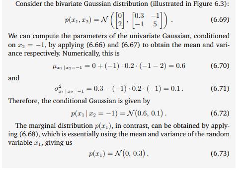
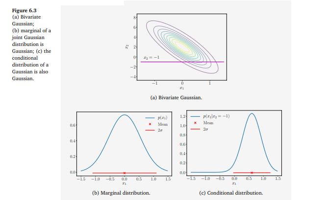
Consider the bivariate Gaussian distribution (illustrated in Figure 6.3): p(x1,2)=N [0.3 ]). (6.69) We can compute the parameters of the univariate Gaussian, conditioned on 2-1, by applying (6.66) and (6.67) to obtain the mean and vari- ance respectively. Numerically, this is and H-10+(-1) 0.2 (-1-2) = 0.6 . (6.70) = 02-10.3-(-1) 0.2 (-1) = 0.1. (6.71) p(x1|2=-1) N(0.6, 0.1). (6.72) Therefore, the conditional Gaussian is given by The marginal distribution p(x1), in contrast, can be obtained by apply- ing (6.68), which is essentially using the mean and variance of the random variable x1, giving us p(x1) = N(0, 0.3). (6.73) Figure 6.3 (a) Bivariate Gaussian; (b) marginal of a joint Gaussian distribution is Gaussian; (c) the conditional distribution of a Gaussian is also Gaussian. 81 61 4 20 0 y=-1 0 (a) Bivariate Gaussian. P) 1.2 p(-1) Mean 0.6 Mean 1.0 20 20 0.8 0.4 0.6 0.44 0.29 0:2 0.0 0.01 -1.5 -1.0 -0.5 0.0 21 0.5 1.0 1.5 -15 -1.0 -0.5 0.0 0.5 1.0 1.5 21 (b) Marginal distribution. (c) Conditional distribution.