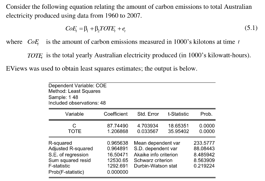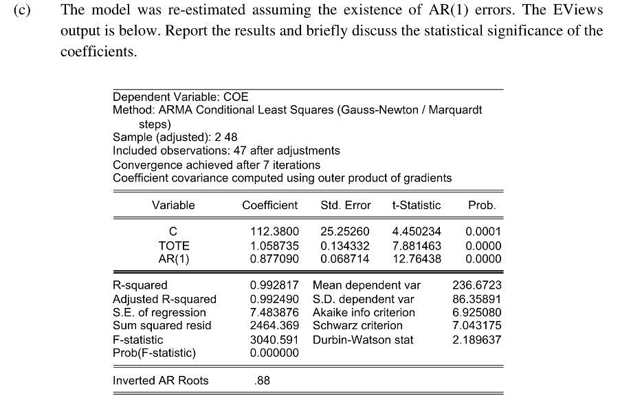


Consider the following equation relating the amount of carbon emissions to total Australian electricity produced using data from 1960 to 2007. CoE, =B. +B TOTE, +e, (5.1) where CoE is the amount of carbon emissions measured in 1000's kilotons at time t TOT is the total yearly Australian electricity produced (in 1000's kilowatt-hours). EViews was used to obtain least squares estimates; the output is below. Dependent Variable: COE Method: Least Squares Sample: 1 48 Included observations: 48 Variable Coefficient Std. Error t-Statistic Prob. TOTE 87.74490 1.206868 4.703934 0.033567 18.65351 35.95402 0.0000 0.0000 R-squared Adjusted R-squared S.E. of regression Sum squared resid F-statistic Prob(F-statistic) 0.965638 Mean dependent var 0.964891 S.D. dependent var 16.50471 Akaike info criterion 12530.65 Schwarz criterion 1292.691 Durbin-Watson stat 233.5777 88.08443 8.485942 8.563909 0.219224 0.000000 (a) Which assumption is violated when the errors are serially correlated? What are the effects of this violation on the least squares estimators? (b) The following EViews output is obtained from a Lagrange Multiplier test for first order serial correlation applied to equation (5.1). Use the Lagrange Multiplier test at the 5 % significance level to test for a first-order autoregressive error. Make sure to specify the null and alternative hypotheses and the test statistic. Breusch-Godfrey Serial Correlation LM Test: 132.4691 F-statistic Obs*R-squared Prob. F(1,45) Prob. Chi-Square(1) 35.82887 (c) The model was re-estimated assuming the existence of AR(1) errors. The EViews output is below. Report the results and briefly discuss the statistical significance of the coefficients. Dependent Variable: COE Method: ARMA Conditional Least Squares (Gauss-Newton / Marquardt steps) Sample (adjusted): 2 48 Included observations: 47 after adjustments Convergence achieved after 7 iterations Coefficient covariance computed using outer product of gradients Variable Coefficient Std. Error t-Statistic Prob. TOTE AR(1) 112.3800 1.058735 0.877090 25.25260 0.134332 0.068714 4.450234 7.881463 12.76438 0.0001 0.0000 0.0000 R-squared Adjusted R-squared S.E. of regression Sum squared resid F-statistic Prob(F-statistic) 0.992817 Mean dependent var 0.992490 S.D. dependent var 7.483876 Akaike info criterion 2464.369 Schwarz criterion 236.6723 86.35891 6.925080 7.043175 2.189637 3040.591 Durbin-Watson stat 0.000000 Inverted AR Roots .88 (d) Forecast carbon emissions for 2008 assuming the value for total electricity produced is 258,000 kilowatt-hours. Find two values for the forecast, one that assumes the errors do not have an autocorrelation problem and one that assumes that they follow an AR(1) process. The levels of carbon emissions and total electricity produced in 2007 were 373.7 and 254.6, respectively. Consider the following equation relating the amount of carbon emissions to total Australian electricity produced using data from 1960 to 2007. CoE, =B. +B TOTE, +e, (5.1) where CoE is the amount of carbon emissions measured in 1000's kilotons at time t TOT is the total yearly Australian electricity produced (in 1000's kilowatt-hours). EViews was used to obtain least squares estimates; the output is below. Dependent Variable: COE Method: Least Squares Sample: 1 48 Included observations: 48 Variable Coefficient Std. Error t-Statistic Prob. TOTE 87.74490 1.206868 4.703934 0.033567 18.65351 35.95402 0.0000 0.0000 R-squared Adjusted R-squared S.E. of regression Sum squared resid F-statistic Prob(F-statistic) 0.965638 Mean dependent var 0.964891 S.D. dependent var 16.50471 Akaike info criterion 12530.65 Schwarz criterion 1292.691 Durbin-Watson stat 233.5777 88.08443 8.485942 8.563909 0.219224 0.000000 (a) Which assumption is violated when the errors are serially correlated? What are the effects of this violation on the least squares estimators? (b) The following EViews output is obtained from a Lagrange Multiplier test for first order serial correlation applied to equation (5.1). Use the Lagrange Multiplier test at the 5 % significance level to test for a first-order autoregressive error. Make sure to specify the null and alternative hypotheses and the test statistic. Breusch-Godfrey Serial Correlation LM Test: 132.4691 F-statistic Obs*R-squared Prob. F(1,45) Prob. Chi-Square(1) 35.82887 (c) The model was re-estimated assuming the existence of AR(1) errors. The EViews output is below. Report the results and briefly discuss the statistical significance of the coefficients. Dependent Variable: COE Method: ARMA Conditional Least Squares (Gauss-Newton / Marquardt steps) Sample (adjusted): 2 48 Included observations: 47 after adjustments Convergence achieved after 7 iterations Coefficient covariance computed using outer product of gradients Variable Coefficient Std. Error t-Statistic Prob. TOTE AR(1) 112.3800 1.058735 0.877090 25.25260 0.134332 0.068714 4.450234 7.881463 12.76438 0.0001 0.0000 0.0000 R-squared Adjusted R-squared S.E. of regression Sum squared resid F-statistic Prob(F-statistic) 0.992817 Mean dependent var 0.992490 S.D. dependent var 7.483876 Akaike info criterion 2464.369 Schwarz criterion 236.6723 86.35891 6.925080 7.043175 2.189637 3040.591 Durbin-Watson stat 0.000000 Inverted AR Roots .88 (d) Forecast carbon emissions for 2008 assuming the value for total electricity produced is 258,000 kilowatt-hours. Find two values for the forecast, one that assumes the errors do not have an autocorrelation problem and one that assumes that they follow an AR(1) process. The levels of carbon emissions and total electricity produced in 2007 were 373.7 and 254.6, respectively
