Question
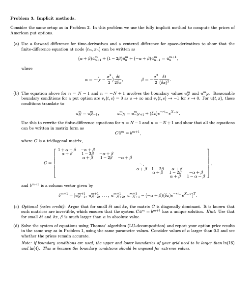
Consider the same setup as in Problem 2. In this problem we use the fully implicit method to compute the prices of American put options.
Consider the same setup as in Problem 2. In this problem we use the fully implicit method to compute the prices of American put options.
(a) Use a forward difference for time-derivatives and a centered difference for space-derivatives to show that the finite-difference equation at node (tm,xn) can be written as
where
(?+?)u ?m +(1?2?)u ?m +(??+?)u ?m
=u ?m+1, n
n+1
n
n?1
?2 ?t ? = ??r ? ?
?2 2 (?x)
2 2?x
,
? = ?
?t
2 .
(b) The equation above for n = N ? 1 and n = ?N + 1 involves the boundary values umN and um?N . Reasonable boundary conditions for a put option are vs(t,s) = 0 as s ? ? and vs(t,s) ? ?1 for s ? 0. For u(t,x), these conditions translate to
umN = umN?1, um?N = um?N+1 + (?x)e?rtm eX?N . Use this to rewrite the finite-difference equations for n = N ? 1 and n = ?N + 1 and show that all the equations
can be written in matrix form as where C is a tridiagonal matrix,
Cu ?m = bm+1,
?1+??? ??+? ? ?+? 1?2? ??+?
? ?+? 1?2? ??+? ? ?.?
C = ? ??
and bm+1 is a column vector given by bm+1 = [u ?m+1, u ?m+1, . . . , u ?m+1
(c) Optional (extra credit): Argue that for small ?t and ?x, the matrix C is diagonally dominant. It is known that such matrices are invertible, which ensures that the system Cu ?m = bm+1 has a unique solution. Hint: Use that for small ?t and ?x, ? is much larger than ? in absolute value.
(d) Solve the system of equations using Thomas' algorithm (LU-decomposition) and report your option price results in the same way as in Problem 1, using the same parameter values. Consider values of ? larger than 0.5 and see whether the prices remain accurate.
Note: if boundary conditions are used, the upper and lower boundaries of your grid need to be larger than ln(16) and ln(4). This is because the boundary conditions should be imposed for extreme values.

Step by Step Solution
There are 3 Steps involved in it
Step: 1

Get Instant Access to Expert-Tailored Solutions
See step-by-step solutions with expert insights and AI powered tools for academic success
Step: 2

Step: 3

Ace Your Homework with AI
Get the answers you need in no time with our AI-driven, step-by-step assistance
Get Started


