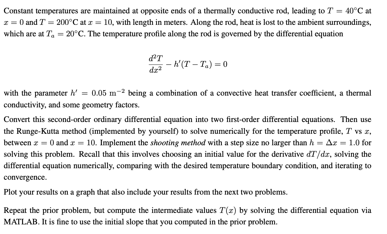
Constant temperatures are maintained at opposite ends of a thermally conductive rod, leading to T=40C at x=0 and T=200C at x=10, with length in meters. Along the rod, heat is lost to the ambient surroundings, which are at Ta=20C. The temperature profile along the rod is governed by the differential equation dx2d2Th(TTa)=0 with the parameter h=0.05m2 being a combination of a convective heat transfer coefficient, a thermal conductivity, and some geometry factors. Convert this second-order ordinary differential equation into two first-order differential equations. Then use the Runge-Kutta method (implemented by yourself) to solve numerically for the temperature profile, T vs x, between x=0 and x=10. Implement the shooting method with a step size no larger than h=x=1.0 for solving this problem. Recall that this involves choosing an initial value for the derivative dT/dx, solving the differential equation numerically, comparing with the desired temperature boundary condition, and iterating to convergence. Plot your results on a graph that also include your results from the next two problems. Repeat the prior problem, but compute the intermediate values T(x) by solving the differential equation via MATLAB. It is fine to use the initial slope that you computed in the prior problem. Constant temperatures are maintained at opposite ends of a thermally conductive rod, leading to T=40C at x=0 and T=200C at x=10, with length in meters. Along the rod, heat is lost to the ambient surroundings, which are at Ta=20C. The temperature profile along the rod is governed by the differential equation dx2d2Th(TTa)=0 with the parameter h=0.05m2 being a combination of a convective heat transfer coefficient, a thermal conductivity, and some geometry factors. Convert this second-order ordinary differential equation into two first-order differential equations. Then use the Runge-Kutta method (implemented by yourself) to solve numerically for the temperature profile, T vs x, between x=0 and x=10. Implement the shooting method with a step size no larger than h=x=1.0 for solving this problem. Recall that this involves choosing an initial value for the derivative dT/dx, solving the differential equation numerically, comparing with the desired temperature boundary condition, and iterating to convergence. Plot your results on a graph that also include your results from the next two problems. Repeat the prior problem, but compute the intermediate values T(x) by solving the differential equation via MATLAB. It is fine to use the initial slope that you computed in the prior