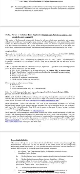
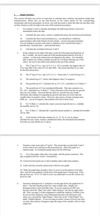
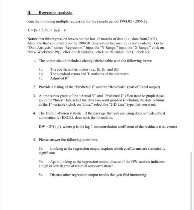
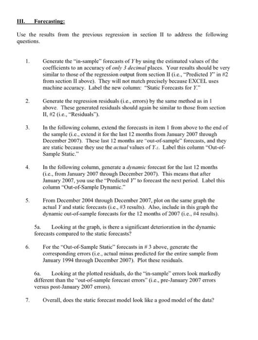
Curiya thala can leave we were e le provide a pedrally Part 2. Review of Statistical Tools Application Submit and Part 3 is Canvas submission PRED The pain of the most is elhelye avec Lillywiled to use when dong the will be and the Colent, and the second toes will be chance with their hands and best sheep www minhas the computer and The data for the case pertenece STA-1_222 TEXCEL file can be The data filee Thee for which The my to De The Es wing only Click on the office Been the per le comer Tarieven Select and the Click to 4. Select Analysis Select Go (in the middle towards beim 6 Check Analysis of box and dete If you wong scarlet veneet Select Tube 2. Ali 1 Schell) Notes For MAC anders who are sign up Add- problem, please follow the instruction below! MS has made it ficut for MAC, including MACB Yeni. The good news for you in the UF Appetom. Po online filme Please note that's the showed beyed to all the which you'll have time w The each stop habe die for End, budeme FC Help 05190PL PT Blick Pese te these virtual deseo we repente, so y gente de local any work that you with desktop will be you wanted here. Yet there for your files tortorget you will want to see your line dayand you feeling in whichever mail med Draph Sima su The time will help you wou were imple data transformatie. Mete Sue Reviewed for the map tory and protectie te hou Data Analysis the freedom of the ForYand can be diely lethed clahate the fine 6 anramadashions that we et celebrado You need to see how this is what pertesh back perinde ac periode Calculate the common Sourt suristial 11 atia wales you remiere at least nalil paira pe as a ' S Hara --- y l Ewel prasim. I Eur. as Aayi lim 1 Factuart, calalar IN Chilalai siras, caretation cetate heat aga period tracked back and pude fack IsCall the cerca 1 lets ashaman Taraities. BEHENS traile a ---- artins. Bear ar alai alalalala 2 The real also TAgas its attiya T * Threa, lag aa N 1. Tenatamil largal. Naalayam 24 The purathiraiearcia s Te pati meal reland areas, - stalin 2 - ruinar y Alanai --- hair, variatile alaraipatine salers TraENE, , dipr.at - * Heater eatialaa ligh the mytale by 12 * Fraurel alelee hapatra pa sakalar dual deities. Note that you did it for the 1 Generate a time series plated and the map waleelai attents are = Inia) Ms. Fernate A. Lalan tarastyai paal anthe ey M. Make the pi Ala, + 106 4 thanE. The title that the late 1 uram has incarnata 2017 - Bestel het terreos - Ne Mr page 2 of aim is it ular at is the re get upuropan" a ne EEL II. Regression Analysis: Run the following multiple regression for the sample period 1994:02 - 2006:12: Y; = Bo + B1Yu + BxX:+ & Notice that this regression leaves out the last 12 months of data (i.e., data from 2007). Also note that you must drop the 1994:01 observation because Y., is not available. Go to "Data Analysis," select "Regression," input the "Y Range," input the "X Range," click on "New Worksheet Ply," click on "Residuals," click on "Residual Plots," click ok. 1. The output should include a clearly labeled table with the following items: The coefficient estimates (i.e., Bo Be, and B2). 1b. The standard errors and T-statistics of the estimates Adjusted R 2. Provide a listing of the "Predicted r" and the "Residuals (part of Excel output) 3. A time series graph of the "Actual Y" and "Predicted r" (You need to graph these go to the "Insert" tab, select the data you want graphed (including the date column as the 1" variable), click on "Line," select the "2-D Line" type that you want. 4. The Durbin Watson statistic. If the package that you are using does not calculate it automatically (EXCEL does not), the formula is: DW = 2*(1-P), where p is the lag-1 autocorrelation coefficient of the residuals (i.e., errors) lc. 5. Please answer the following questions: Sa. Looking at the regression output, explain which coefficients are statistically significant 5b. Again looking at the regression output, discuss if the DW statistic indicates a high or low degree of residual autocorrelation? Sc. Discuss other regression output results that you find interesting. III. Forecasting: Use the results from the previous regression in section Il to address the following questions. 1. 2. 3. Generate the "in-sample" forecasts of Y by using the estimated values of the coefficients to an accuracy of only 3 decimal places. Your results should be very similar to those of the regression output from section II (i.e., "Predicted "in #2 from section II above). They will not match precisely because EXCEL uses machine accuracy. Label the new column: Static Forecasts for Y." Generate the regression residuals (i.e., errors) by the same method as in 1 above. These generated residuals should again be similar to those from section II, #2 (i.e., "Residuals"). In the following column, extend the forecasts in item 1 from above to the end of the sample (i.e., extend it for the last 12 months from January 2007 through December 2007). These last 12 months are "out-of-sample" forecasts, and they are static because they use the actual values of Y... Label this column "Out-of- Sample Static." In the following column, generate a dynamic forecast for the last 12 months (i.c., from January 2007 through December 2007). This means that after January 2007, you use the "Predicted Y" to forecast the next period. Label this column "Out-of-Sample Dynamic." From December 2004 through December 2007, plot on the same graph the actual Y and static forecasts (i.e., #3 results). Also, include in this graph the dynamic out-of-sample forecasts for the 12 months of 2007 (i.e., #4 results). 5a. Looking at the graph, is there a significant deterioration in the dynamic forecasts compared to the static forecasts? For the "Out-of-Sample Static" forecasts in # 3 above, generate the corresponding errors (i.c., actual minus predicted for the entire sample from January 1994 through December 2007). Plot these residuals. . Looking at the plotted residuals, do the "in-sample" errors look markedly different than the "out-of-sample forecast errors" (i.c., pre-January 2007 errors versus post January 2007 errors). Overall, does the static forecast model look like a good model of the data? 5. 6. 7. Curiya thala can leave we were e le provide a pedrally Part 2. Review of Statistical Tools Application Submit and Part 3 is Canvas submission PRED The pain of the most is elhelye avec Lillywiled to use when dong the will be and the Colent, and the second toes will be chance with their hands and best sheep www minhas the computer and The data for the case pertenece STA-1_222 TEXCEL file can be The data filee Thee for which The my to De The Es wing only Click on the office Been the per le comer Tarieven Select and the Click to 4. Select Analysis Select Go (in the middle towards beim 6 Check Analysis of box and dete If you wong scarlet veneet Select Tube 2. Ali 1 Schell) Notes For MAC anders who are sign up Add- problem, please follow the instruction below! MS has made it ficut for MAC, including MACB Yeni. The good news for you in the UF Appetom. Po online filme Please note that's the showed beyed to all the which you'll have time w The each stop habe die for End, budeme FC Help 05190PL PT Blick Pese te these virtual deseo we repente, so y gente de local any work that you with desktop will be you wanted here. Yet there for your files tortorget you will want to see your line dayand you feeling in whichever mail med Draph Sima su The time will help you wou were imple data transformatie. Mete Sue Reviewed for the map tory and protectie te hou Data Analysis the freedom of the ForYand can be diely lethed clahate the fine 6 anramadashions that we et celebrado You need to see how this is what pertesh back perinde ac periode Calculate the common Sourt suristial 11 atia wales you remiere at least nalil paira pe as a ' S Hara --- y l Ewel prasim. I Eur. as Aayi lim 1 Factuart, calalar IN Chilalai siras, caretation cetate heat aga period tracked back and pude fack IsCall the cerca 1 lets ashaman Taraities. BEHENS traile a ---- artins. Bear ar alai alalalala 2 The real also TAgas its attiya T * Threa, lag aa N 1. Tenatamil largal. Naalayam 24 The purathiraiearcia s Te pati meal reland areas, - stalin 2 - ruinar y Alanai --- hair, variatile alaraipatine salers TraENE, , dipr.at - * Heater eatialaa ligh the mytale by 12 * Fraurel alelee hapatra pa sakalar dual deities. Note that you did it for the 1 Generate a time series plated and the map waleelai attents are = Inia) Ms. Fernate A. Lalan tarastyai paal anthe ey M. Make the pi Ala, + 106 4 thanE. The title that the late 1 uram has incarnata 2017 - Bestel het terreos - Ne Mr page 2 of aim is it ular at is the re get upuropan" a ne EEL II. Regression Analysis: Run the following multiple regression for the sample period 1994:02 - 2006:12: Y; = Bo + B1Yu + BxX:+ & Notice that this regression leaves out the last 12 months of data (i.e., data from 2007). Also note that you must drop the 1994:01 observation because Y., is not available. Go to "Data Analysis," select "Regression," input the "Y Range," input the "X Range," click on "New Worksheet Ply," click on "Residuals," click on "Residual Plots," click ok. 1. The output should include a clearly labeled table with the following items: The coefficient estimates (i.e., Bo Be, and B2). 1b. The standard errors and T-statistics of the estimates Adjusted R 2. Provide a listing of the "Predicted r" and the "Residuals (part of Excel output) 3. A time series graph of the "Actual Y" and "Predicted r" (You need to graph these go to the "Insert" tab, select the data you want graphed (including the date column as the 1" variable), click on "Line," select the "2-D Line" type that you want. 4. The Durbin Watson statistic. If the package that you are using does not calculate it automatically (EXCEL does not), the formula is: DW = 2*(1-P), where p is the lag-1 autocorrelation coefficient of the residuals (i.e., errors) lc. 5. Please answer the following questions: Sa. Looking at the regression output, explain which coefficients are statistically significant 5b. Again looking at the regression output, discuss if the DW statistic indicates a high or low degree of residual autocorrelation? Sc. Discuss other regression output results that you find interesting. III. Forecasting: Use the results from the previous regression in section Il to address the following questions. 1. 2. 3. Generate the "in-sample" forecasts of Y by using the estimated values of the coefficients to an accuracy of only 3 decimal places. Your results should be very similar to those of the regression output from section II (i.e., "Predicted "in #2 from section II above). They will not match precisely because EXCEL uses machine accuracy. Label the new column: Static Forecasts for Y." Generate the regression residuals (i.e., errors) by the same method as in 1 above. These generated residuals should again be similar to those from section II, #2 (i.e., "Residuals"). In the following column, extend the forecasts in item 1 from above to the end of the sample (i.e., extend it for the last 12 months from January 2007 through December 2007). These last 12 months are "out-of-sample" forecasts, and they are static because they use the actual values of Y... Label this column "Out-of- Sample Static." In the following column, generate a dynamic forecast for the last 12 months (i.c., from January 2007 through December 2007). This means that after January 2007, you use the "Predicted Y" to forecast the next period. Label this column "Out-of-Sample Dynamic." From December 2004 through December 2007, plot on the same graph the actual Y and static forecasts (i.e., #3 results). Also, include in this graph the dynamic out-of-sample forecasts for the 12 months of 2007 (i.e., #4 results). 5a. Looking at the graph, is there a significant deterioration in the dynamic forecasts compared to the static forecasts? For the "Out-of-Sample Static" forecasts in # 3 above, generate the corresponding errors (i.c., actual minus predicted for the entire sample from January 1994 through December 2007). Plot these residuals. . Looking at the plotted residuals, do the "in-sample" errors look markedly different than the "out-of-sample forecast errors" (i.c., pre-January 2007 errors versus post January 2007 errors). Overall, does the static forecast model look like a good model of the data? 5. 6. 7
