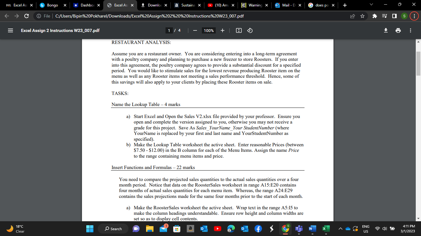
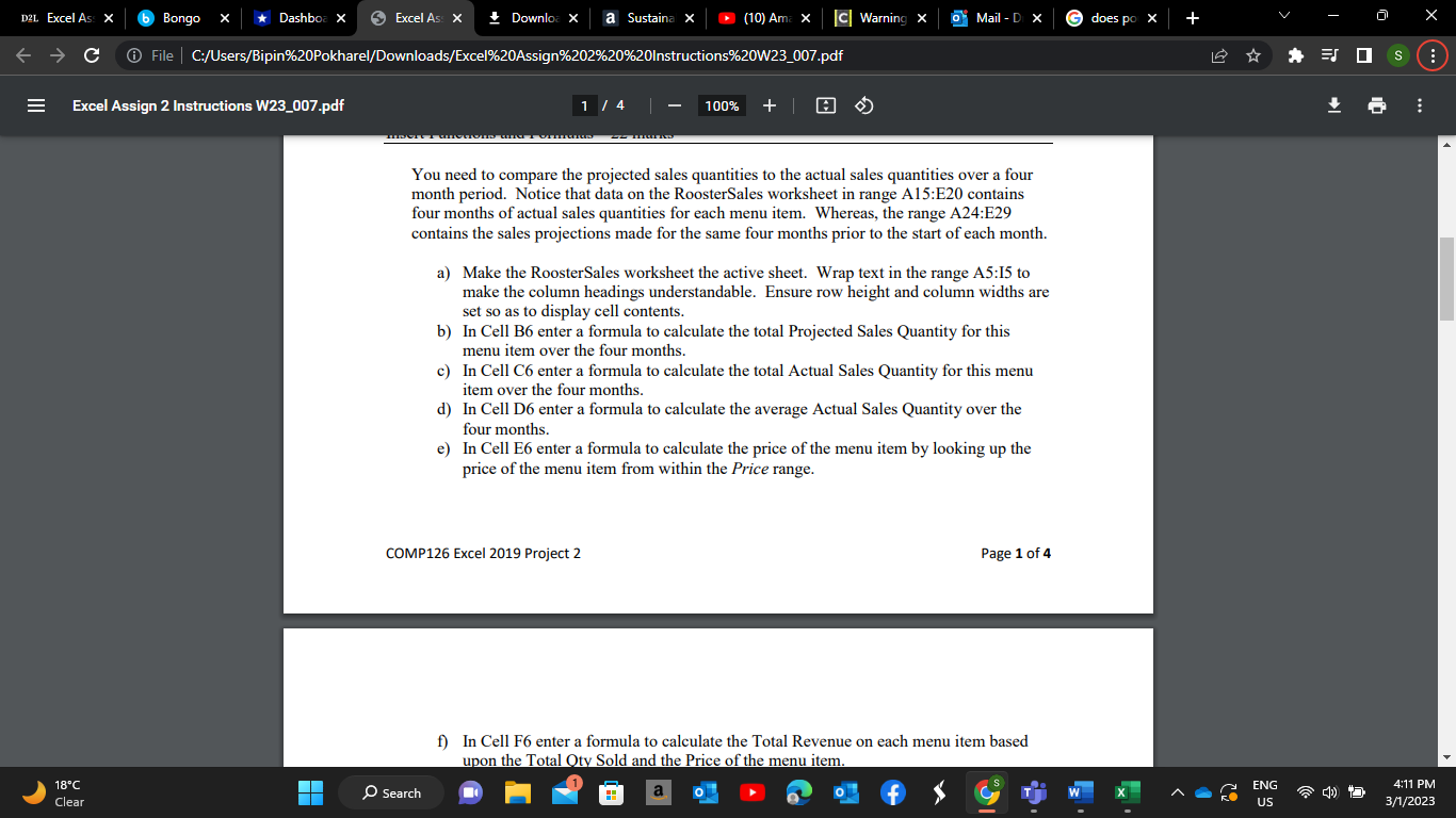
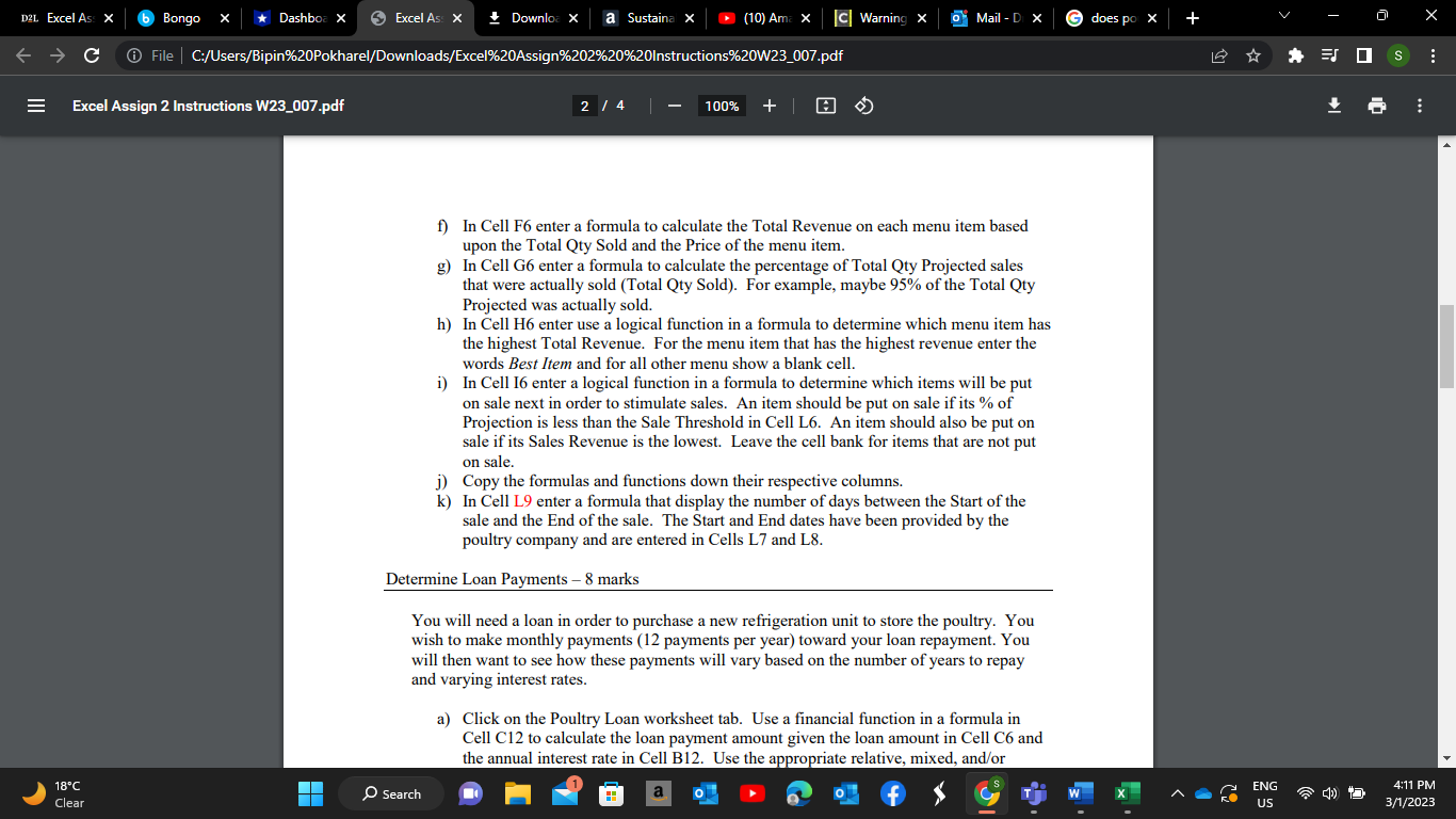
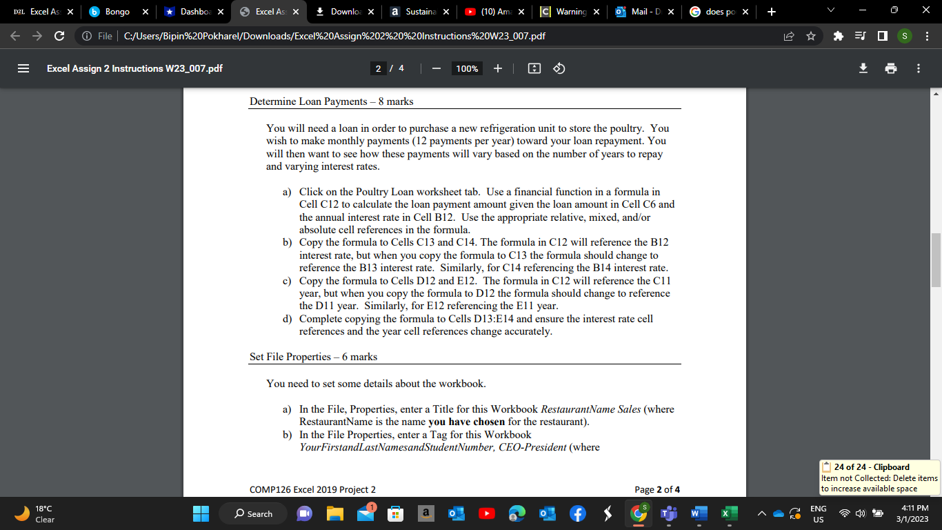
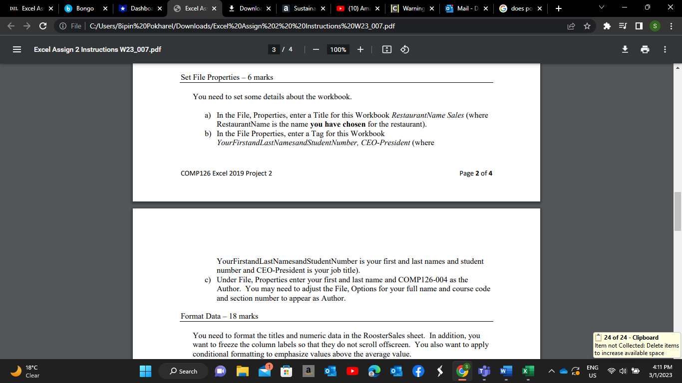
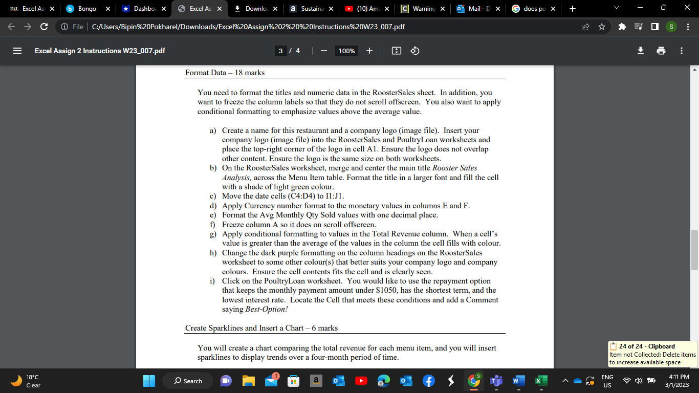
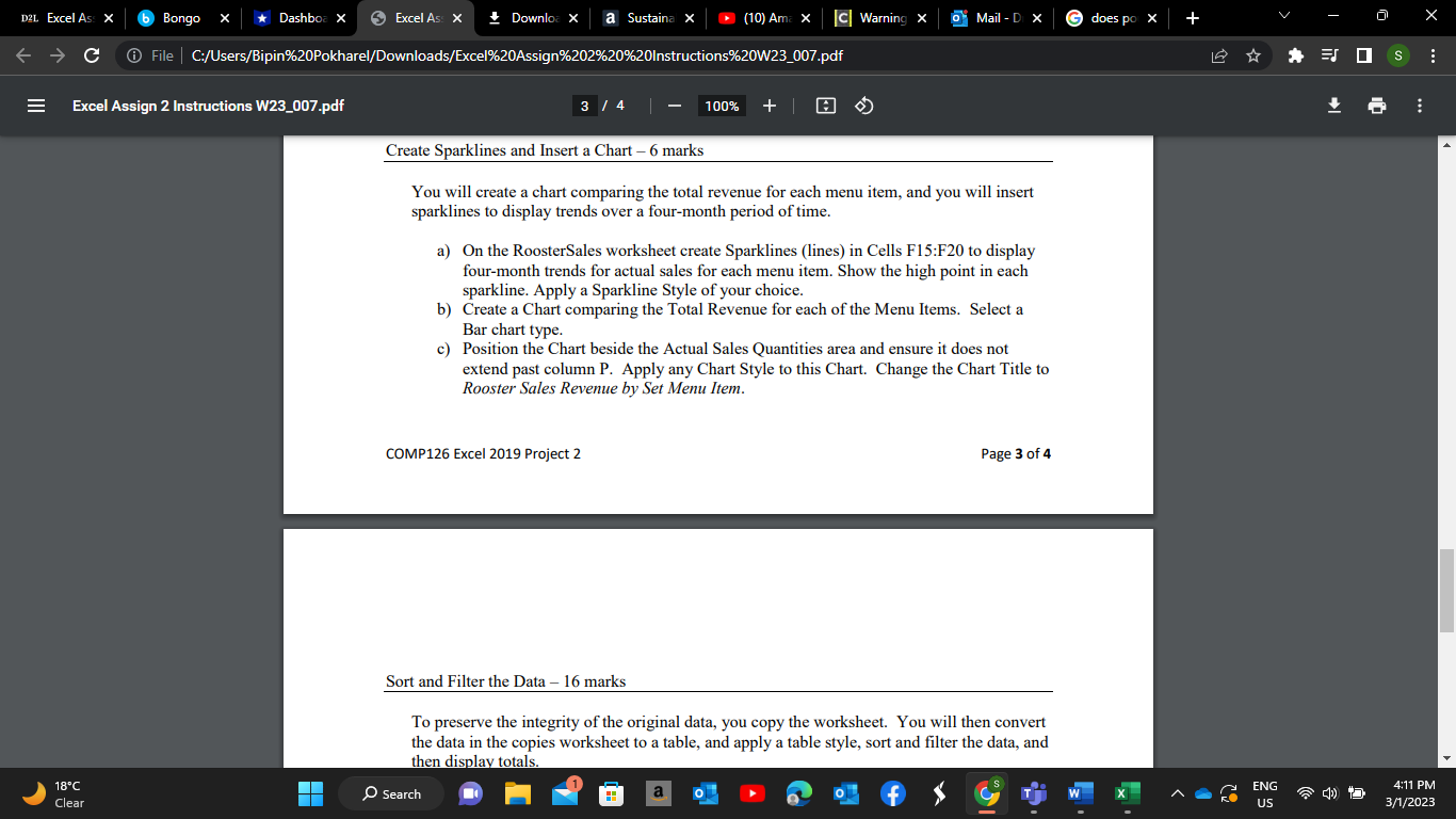
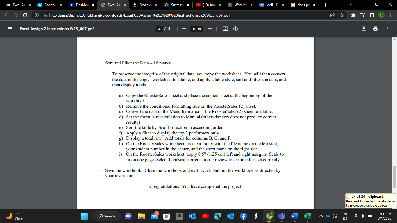
D2L Excel Ass X Bongo X Dashboa X Excel Ass X Downloa X a Sustainal X (10) Ama x C Warning X Mail - Di X does por X + File C:/Users/Bipin%20Pokharel/Downloads/Excel%20Assign%202%20%20Instructions%20W23_007.pdf Excel Assign 2 Instructions W23_007.pdf 1/4 100% + RESTAURANT ANALYSIS: Assume you are a restaurant owner. You are considering entering into a long-term agreement with a poultry company and planning to purchase a new freezer to store Roosters. If you enter into this agreement, the poultry company agrees to provide a substantial discount for a specified period. You would like to stimulate sales for the lowest revenue producing Rooster item on the menu as well as any Rooster items not meeting a sales performance threshold. Hence, some of this savings will also apply to your clients by placing these Rooster items on sale. TASKS: Name the Lookup Table - 4 marks a) Start Excel and Open the Sales V2.xlsx file provided by your professor. Ensure you open and complete the version assigned to you, otherwise you may not receive a grade for this project. Save As Sales_YourName Your Student Number (where YourName is replaced by your first and last name and YourStudent Number as specified). b) Make the Lookup Table worksheet the active sheet. Enter reasonable Prices (between $7.50 - $12.00) in the B column for each of the Menu Items. Assign the name Price to the range containing menu items and price. Insert Functions and Formulas - 22 marks You need to compare the projected sales quantities to the actual sales quantities over a four month period. Notice that data on the RoosterSales worksheet in range A15:E20 contains four months of actual sales quantities for each menu item. Whereas, the range A24:E29 contains the sales projections made for the same four months prior to the start of each month. 18C Search Clear a) Make the RoosterSales worksheet the active sheet. Wrap text in the range A5:15 to make the column headings understandable. Ensure row height and column widths are set so as to display cell contents. a ENG US 4:11 PM 3/1/2023 D2L Excel Ass X Bongo X Dashboa X Excel Ass X Downloa X a Sustainal X (10) Ama x C Warning X Mail - Di X does por X + File C:/Users/Bipin%20Pokharel/Downloads/Excel%20Assign%202%20%20Instructions%20W23_007.pdf Excel Assign 2 Instructions W23_007.pdf 1 / 4 100% You need to compare the projected sales quantities to the actual sales quantities over a four month period. Notice that data on the RoosterSales worksheet in range A15:E20 contains four months of actual sales quantities for each menu item. Whereas, the range A24:E29 contains the sales projections made for the same four months prior to the start of each month. a) Make the RoosterSales worksheet the active sheet. Wrap text in the range A5:15 to make the column headings understandable. Ensure row height and column widths are set so as to display cell contents. b) In Cell B6 enter a formula to calculate the total Projected Sales Quantity for this menu item over the four months. c) In Cell C6 enter a formula to calculate the total Actual Sales Quantity for this menu item over the four months. d) In Cell D6 enter a formula to calculate the average Actual Sales Quantity over the four months. e) In Cell E6 enter a formula to calculate the price of the menu item by looking up the price of the menu item from within the Price range. COMP126 Excel 2019 Project 2 18C Clear Search Page 1 of 4 f) In Cell F6 enter a formula to calculate the Total Revenue on each menu item based upon the Total Oty Sold and the Price of the menu item. a ENG US 4:11 PM 3/1/2023 18C Clear D2L Excel Ass X Bongo X Dashboa X Excel Ass X Downloa X a Sustainal X (10) Ama x C Warning X Mail - Di X does por X + File C:/Users/Bipin%20Pokharel/Downloads/Excel%20Assign%202%20%20Instructions%20W23_007.pdf Excel Assign 2 Instructions W23_007.pdf 2/4 100% +| H f) In Cell F6 enter a formula to calculate the Total Revenue on each menu item based upon the Total Qty Sold and the Price of the menu item. g) In Cell G6 enter a formula to calculate the percentage of Total Qty Projected sales that were actually sold (Total Qty Sold). For example, maybe 95% of the Total Qty Projected was actually sold. h) In Cell H6 enter use a logical function in a formula to determine which menu item has the highest Total Revenue. For the menu item that has the highest revenue enter the words Best Item and for all other menu show a blank cell. i) In Cell 16 enter a logical function in a formula to determine which items will be put on sale next in order to stimulate sales. An item should be put on sale if its % of Projection is less than the Sale Threshold in Cell L6. An item should also be put on sale if its Sales Revenue is the lowest. Leave the cell bank for items that are not put on sale. j) Copy the formulas and functions down their respective columns. k) In Cell L9 enter a formula that display the number of days between the Start of the sale and the End of the sale. The Start and End dates have been provided by the poultry company and are entered in Cells L7 and L8. Determine Loan Payments - 8 marks You will need a loan in order to purchase a new refrigeration unit to store the poultry. You wish to make monthly payments (12 payments per year) toward your loan repayment. You will then want to see how these payments will vary based on the number of years to repay and varying interest rates. O Search a) Click on the Poultry Loan worksheet tab. Use a financial function in a formula in Cell C12 to calculate the loan payment amount given the loan amount in Cell C6 and the annual interest rate in Cell B12. Use the appropriate relative, mixed, and/or a ENG US 4:11 PM 3/1/2023 D2L Excel Ass X Bongo X Dashboa X Excel Ass X Downloa X a Sustainal X (10) Ama x C Warning X Mail - Di X does por X + File C:/Users/Bipin%20Pokharel/Downloads/Excel%20Assign%202%20%20Instructions%20W23_007.pdf Excel Assign 2 Instructions W23_007.pdf 18C Clear 2/4 100% + Determine Loan Payments - 8 marks You will need a loan in order to purchase a new refrigeration unit to store the poultry. You wish to make monthly payments (12 payments per year) toward your loan repayment. You will then want to see how these payments will vary based on the number of years to repay and varying interest rates. a) Click on the Poultry Loan worksheet tab. Use a financial function in a formula in Cell C12 to calculate the loan payment amount given the loan amount in Cell C6 and the annual interest rate in Cell B12. Use the appropriate relative, mixed, and/or absolute cell references in the formula. b) Copy the formula to Cells C13 and C14. The formula in C12 will reference the B12 interest rate, but when you copy the formula to C13 the formula should change to reference the B13 interest rate. Similarly, for C14 referencing the B14 interest rate. c) Copy the formula to Cells D12 and E12. The formula in C12 will reference the C11 year, but when you copy the formula to D12 the formula should change to reference the D11 year. Similarly, for E12 referencing the E11 year. d) Complete copying the formula to Cells D13:E14 and ensure the interest rate cell references and the year cell references change accurately. Set File Properties - 6 marks You need to set some details about the workbook. a) In the File, Properties, enter a Title for this Workbook RestaurantName Sales (where RestaurantName is the name you have chosen for the restaurant). b) In the File Properties, enter a Tag for this Workbook YourFirstandLastNamesandStudentNumber, CEO-President (where COMP126 Excel 2019 Project 2 Search a 24 of 24 - Clipboard Item not Collected: Delete items to increase available space Page 2 of 4 ENG US 4:11 PM 3/1/2023 D2L Excel Ass X Bongo X Dashboa X Excel Ass X Downloa X a Sustainal X (10) Ama x C Warning X Mail - Di X does por X + File C:/Users/Bipin%20Pokharel/Downloads/Excel%20Assign%202%20%20Instructions%20W23_007.pdf Excel Assign 2 Instructions W23_007.pdf Set File Properties - 6 marks 3/4 100% + | You need to set some details about the workbook. a) In the File, Properties, enter a Title for this Workbook RestaurantName Sales (where RestaurantName is the name you have chosen for the restaurant). b) In the File Properties, enter a Tag for this Workbook YourFirstandLastNamesandStudentNumber, CEO-President (where COMP126 Excel 2019 Project 2 Page 2 of 4 YourFirstandLastNamesandStudentNumber is your first and last names and student number and CEO-President is your job title). c) Under File, Properties enter your first and last name and COMP126-004 as the Author. You may need to adjust the File, Options for your full name and course code and section number to appear as Author. Format Data 18 marks You need to format the titles and numeric data in the RoosterSales sheet. In addition, you want to freeze the column labels so that they do not scroll offscreen. You also want to apply conditional formatting to emphasize values above the average value. a 18C Clear O Search 24 of 24 - Clipboard Item not Collected: Delete items to increase available space ENG US 4:11 PM 3/1/2023 D2L Excel Ass X Bongo X Dashboa X Excel Ass X Downloa X a Sustainal X (10) Ama x C Warning X Mail - Di X does por X + File C:/Users/Bipin%20Pokharel/Downloads/Excel%20Assign%202%20%20Instructions%20W23_007.pdf Excel Assign 2 Instructions W23_007.pdf Format Data 18 marks 3 / 4 100% + | You need to format the titles and numeric data in the RoosterSales sheet. In addition, you want to freeze the column labels so that they do not scroll offscreen. You also want to apply conditional formatting to emphasize values above the average value. a) Create a name for this restaurant and a company logo (image file). Insert your company logo (image file) into the RoosterSales and Poultry Loan worksheets and place the top-right corner of the logo in cell A1. Ensure the logo does not overlap other content. Ensure the logo is the same size on both worksheets. b) On the RoosterSales worksheet, merge and center the main title Rooster Sales Analysis, across the Menu Item table. Format the title in a larger font and fill the cell with a shade of light green colour. c) Move the date cells (C4:D4) to 11:J1. d) Apply Currency number format to the monetary values in columns E and F. e) Format the Avg Monthly Qty Sold values with one decimal place. f) Freeze column A so it does on scroll offscreen. g) Apply conditional formatting to values in the Total Revenue column. When a cell's value is greater than the average of the values in the column the cell fills with colour. h) Change the dark purple formatting on the column headings on the RoosterSales worksheet to some other colour(s) that better suits your company logo and company colours. Ensure the cell contents fits the cell and is clearly seen. i) Click on the PoultryLoan worksheet. You would like to use the repayment option that keeps the monthly payment amount under $1050, has the shortest term, and the lowest interest rate. Locate the Cell that meets these conditions and add a Comment saying Best-Option! Create Sparklines and Insert a Chart - 6 marks You will create a chart comparing the total revenue for each menu item, and you will insert sparklines to display trends over a four-month period of time. 18C Clear Search a 24 of 24 - Clipboard Item not Collected: Delete items to increase available space ENG US 4:11 PM 3/1/2023 D2L Excel Ass X Bongo X Dashboa X Excel Ass X Downloa X a Sustainal X (10) Ama x C Warning X Mail - Di X does por X + File C:/Users/Bipin%20Pokharel/Downloads/Excel%20Assign%202%20%20Instructions%20W23_007.pdf Excel Assign 2 Instructions W23_007.pdf 3/4 100% Create Sparklines and Insert a Chart - 6 marks You will create a chart comparing the total revenue for each menu item, and you will insert sparklines to display trends over a four-month period of time. a) On the RoosterSales worksheet create Sparklines (lines) in Cells F15:F20 to display four-month trends for actual sales for each menu item. Show the high point in each sparkline. Apply a Sparkline Style of your choice. b) Create a Chart comparing the Total Revenue for each of the Menu Items. Select a Bar chart type. c) Position the Chart beside the Actual Sales Quantities area and ensure it does not extend past column P. Apply any Chart Style to this Chart. Change the Chart Title to Rooster Sales Revenue by Set Menu Item. COMP126 Excel 2019 Project 2 Page 3 of 4 Sort and Filter the Data - 16 marks To preserve the integrity of the original data, you copy the worksheet. You will then convert the data in the copies worksheet to a table, and apply a table style, sort and filter the data, and then display totals. 18C O Search Clear a ENG US 4:11 PM 3/1/2023 D2L Excel Ass X Bongo X Dashboa X Excel Ass X Downloa X a Sustainal X (10) Ama x C Warning X Mail - Di X does por X + File C:/Users/Bipin%20Pokharel/Downloads/Excel%20Assign%202%20%20Instructions%20W23_007.pdf Excel Assign 2 Instructions W23_007.pdf 4 / 4 100% +| Sort and Filter the Data - 16 marks To preserve the integrity of the original data, you copy the worksheet. You will then convert the data in the copies worksheet to a table, and apply a table style, sort and filter the data, and then display totals. a) Copy the RoosterSales sheet and place the copied sheet at the beginning of the workbook. b) Remove the conditional formatting rule on the RoosterSales (2) sheet. c) Convert the data in the Menu Item area in the RoosterSales (2) sheet to a table. d) Set the formula recalculation to Manual (otherwise sort does not produce correct results) e) Sort the table by % of Projection in ascending order. f) Apply a filter to display the top 2 performers only. g) Display a total row. Add totals for columns B, C, and F. h) On the RoosterSales worksheet, create a footer with the file name on the left side, your student number in the center, and the sheet name on the right side. i) On the RoosterSales worksheet, apply 0.5" (1.25 cm) left and right margins. Scale to fit on one page. Select Landscape orientation. Preview to ensure all is set correctly. Save the workbook. Close the workbook and exit Excel. Submit the workbook as directed by your instructor. Congratulations! You have completed the project. 18C Clear O Search a 24 of 24 - Clipboard Item not Collected: Delete items to increase available space ENG W US 4:11 PM 3/1/2023