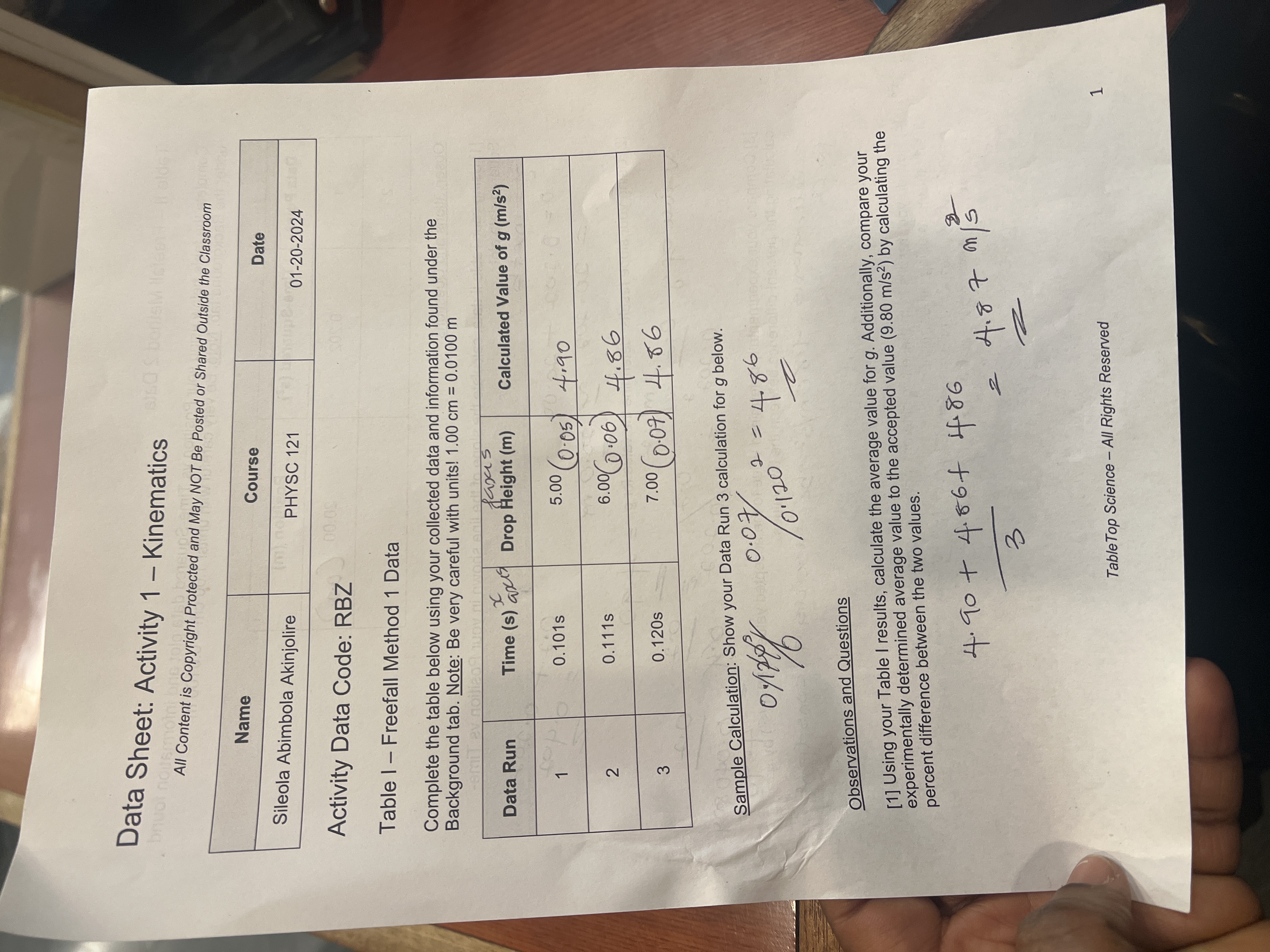
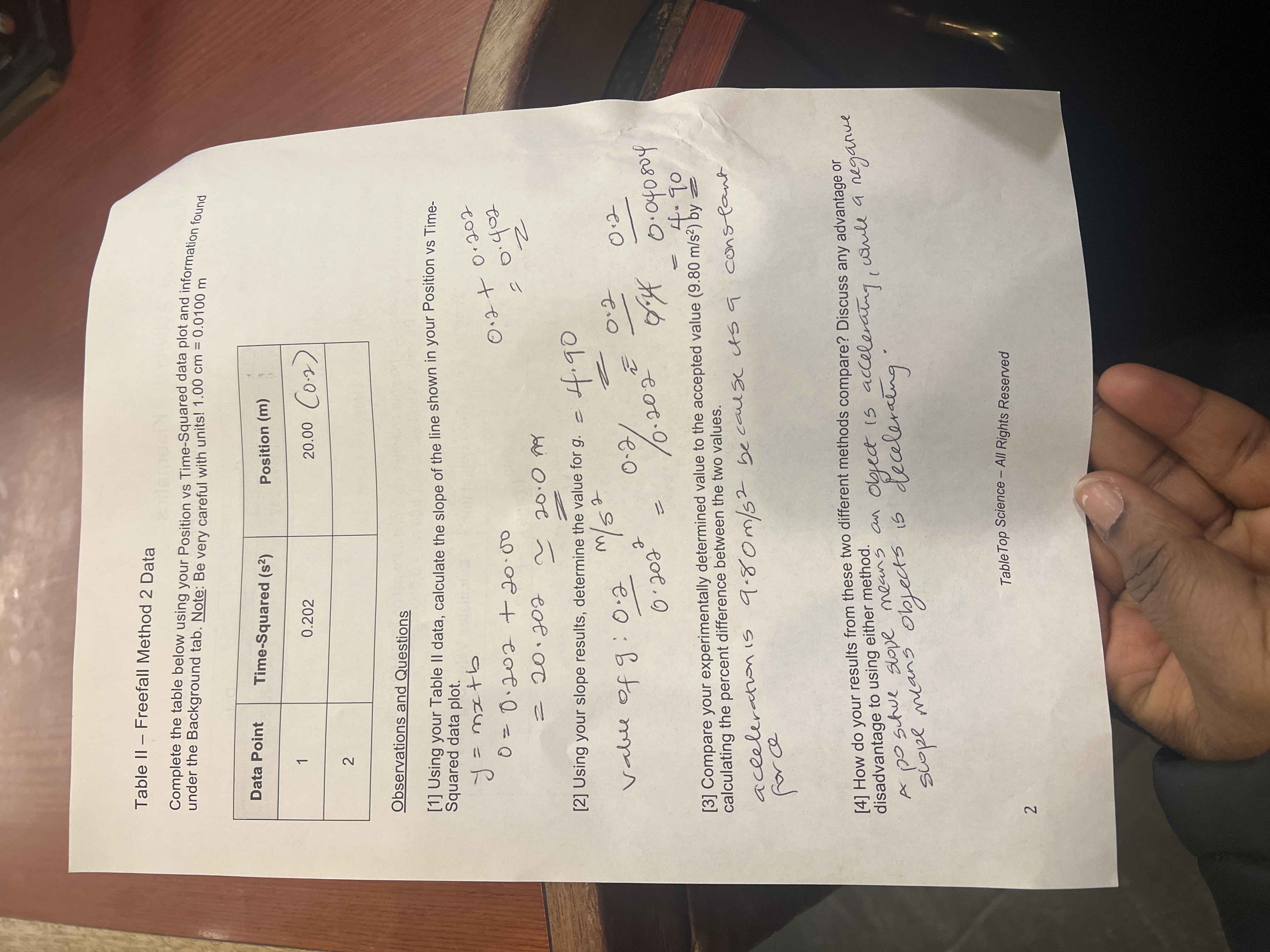
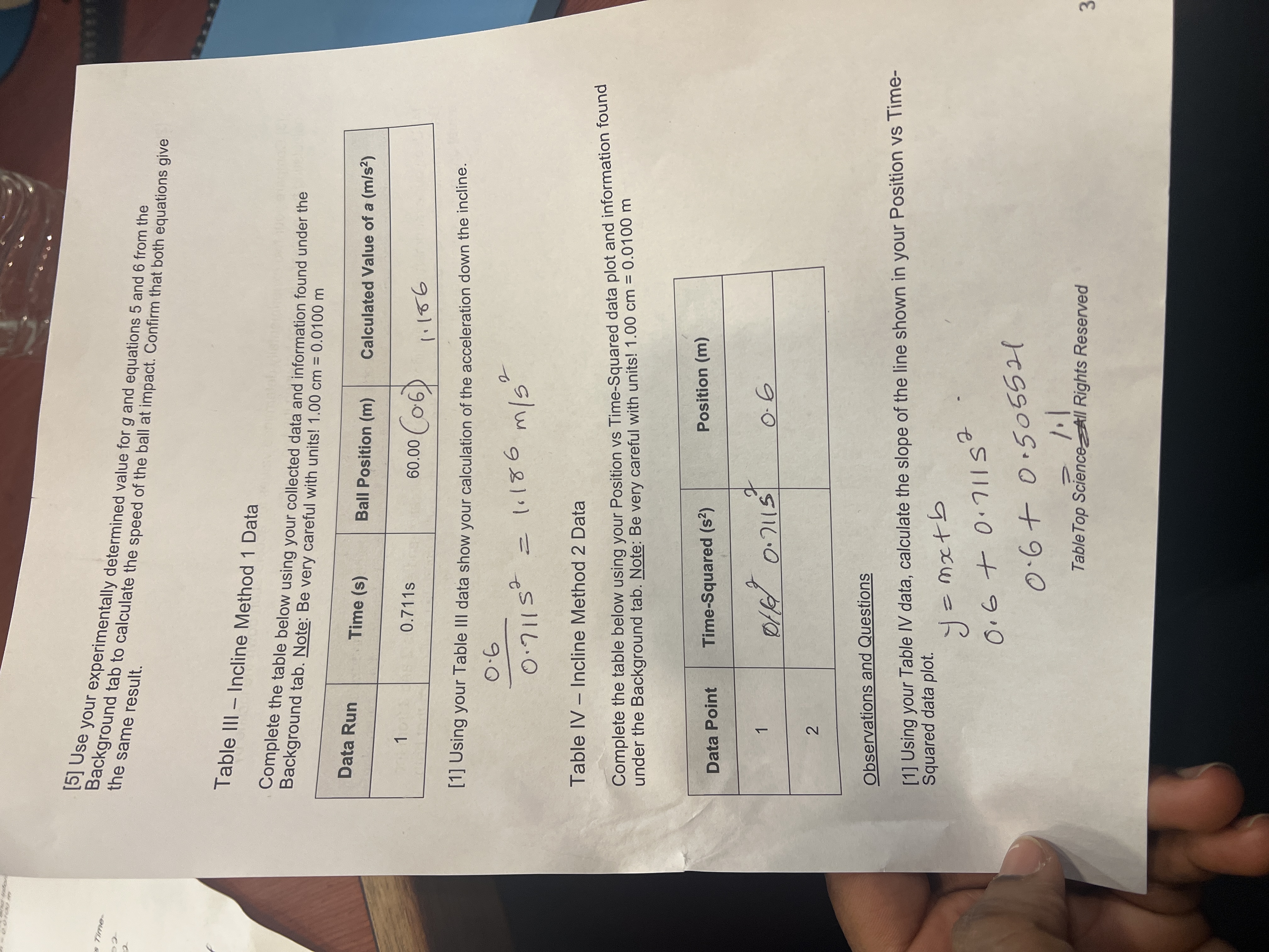
Data Sheet: Activity 1 - Kinematics buot noismo ht Prof All Content is Copyright Protected and May NOT Be Posted or Shared Outside the Classroom Name Course Sileola Abimbola Akinjolire PHYSC 121 00:09 Activity Data Code: RBZ Date 01-20-2024 Table 1 - Freefall Method 1 Data Complete the table below using your collected data and information found under the Background tab. Note: Be very careful with units! 1.00 cm = 0.0100 m Data Run Time (s) x axis faxas Drop Height (m) Calculated Value of g (m/s) 1 0.101s 5.00 (0.05) 4.90 0.111s 2 6.00 (0.06) 4.86 3 0.120s 7.00 (0.07) 4.86 Sample Calculation: Show your Data Run 3 calculation for g below. 0.07 2 = = 4.86 01/1796 /0-1202 Observations and Questions [1] Using your Table I results, calculate the average value for g. Additionally, compare your experimentally determined average value to the accepted value (9.80 m/s) by calculating the percent difference between the two values. 4.90 +4.86+ 4.86. 3 2 4.87 m/s Table Top Science - All Rights Reserved 1 Table II - Freefall Method 2 Data under the Background tab. Note: Be very careful with units! 1.00 cm = 0.0100 m Complete the table below using your Position vs Time-Squared data plot and information found Data Point Time-Squared (s2) Position (m) 1 0.202 20.00 (0.2) 2 [2] Using your slope results, determine the value for g. - Observations and Questions [1] Using your Table II data, calculate the slope of the line shown in your Position vs Time- Squared data plot. =mx+b = 20.202 0=0202 +20.00 0.2+0.202 20.09 = 0.402 2 vable of 9: 0.2 m/s 2 4.90 2 0.202 0.0.202 0.2 0.2 0.20.2 0.4 0.040804 4.90 [3] Compare your experimentally determined value to the accepted value (9.80 m/s) by calculating the percent difference between the two values. acceleration is 9.80m/52 because its a constant for c [4] How do your results from these two different methods compare? Discuss any advantage or disadvantage to using either method. A po Schue slope means an object is accelerating, while a negative scope means objects is decelerating is 2 Table Top Science - All Rights Reserved s Time- [5] Use your experimentally determined value for g and equations 5 and 6 from the Background tab to calculate the speed of the ball at impact. Confirm that both equations give the same result. Table III - Incline Method 1 Data Complete the table below using your collected data and information found under the Background tab. Note: Be very careful with units! 1.00 cm = 0.0100 m Data Run Time (s) Ball Position (m) Calculated Value of a (m/s) 1 0.711s 60.00 (0.6) 1.186 [1] Using your Table III data show your calculation of the acceleration down the incline. 0.6 0.71152 = 1.186 2 m/s Table IV - Incline Method 2 Data Complete the table below using your Position vs Time-Squared data plot and information found under the Background tab. Note: Be very careful with units! 1.00 cm = 0.0100 m Data Point Time-Squared (s) Position (m) 1 0114 0.7115 0.6 2 Observations and Questions [1] Using your Table IV data, calculate the slope of the line shown in your Position vs Time- Squared data plot. y = mx+b 2 0.6+0.711S 0.6+0.505521 1.1 Table Top Science All Rights Reserved 3 [2] Using your slope results, determine the value for a. Journal [3] Compare your two experimentally determined values for acceleration down the incline by calculating the percent difference between the two values. [4] Use your experimentally determined value for acceleration and equations 2 and 3 from the Background tab to calculate the speed of the ball at the end of the data run. Confirm that both equations give the same result. Table Top Science - All Rights Reserved