***data.csv***

**lin_reg.py**

import numpy as np import pandas as pd import matplotlib.pyplot as plt

# function name: least_sq # inputs: file_name- name of the csv file # output: m(slope), b(y-intercept) (IN THAT EXACT ORDER!!!) # LITERALLY return m, b (both rounded 4 decimal places) # YOU HAVE BEEN WARNED! YOU WILL GET IT WRONG IF YOU DO NOT RETURN THE CORRECT THINGS IN THE CORRECT ORDER!!!! # assumptions: The csv file will always have headers in the order of: x, y def least_sq(file_name): pass

# function name: mat_least_sq # inputs: file_name- name of the csv file # output: m (slope), b(y-intercept) (IN THAT EXACT ORDER!!!) # LITERALLY return m, b (both rounded 4 decimal places) # YOU HAVE BEEN WARNED! YOU WILL GET IT WRONG IF YOU DO NOT RETURN THE CORRECT THINGS IN THE CORRECT ORDER! # assumptions: The csv file will always have headers in the order of: x, y def mat_least_sq(file_name): pass

# function name: predict # inputs: file_name- name of the csv file # x- input value that you will interpolate or extrapolate using mat_least_sq # output: the predicted value based on the linear regression equation found using mat_least_sq # The output should be rounded to 4 decimal places # assumptions: The csv file will always have headers in the order of: x, y def predict(file_name, x): pass

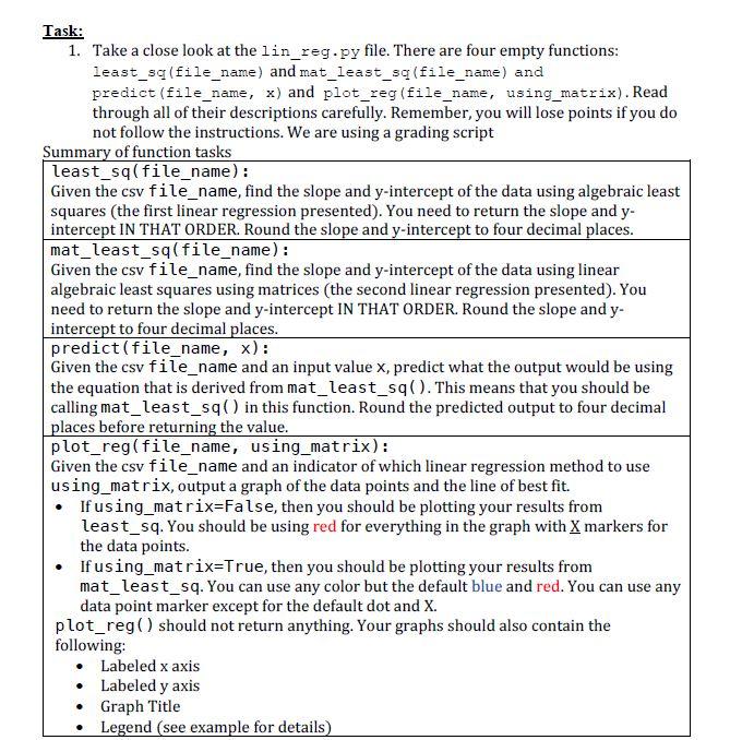
# function name: plot_reg # inputs: file_name- name of the csv file # using_matrix: True if you are plotting the linear equation from mat_least_sq # False if you are plotting the linear equation from least_sq # output: nothing is returned # task: given file_name, compute the linear equation using least_sq or mat_least_sq and graph results # your graph should have the following: labeled x and y axes, title, legend # if using_matrix is False (using least_sq), use X's and red in your graph # if using_matrix is True (using mat_least_sq), you can use any color except for the default blue and red # you can use any marker except for the default dot and X # assumptions: The csv file will always have headers in the order of: x, y def plot_reg(file_name, using_matrix): pass

######## TEST CASES ######## # this test case is the same as the one in csv_file = "data.csv"

m1, b1 = least_sq(csv_file) print("Slope using algebraic least squares:", m1) print("y-intercept using algebraic least squares:", b1) print()

m2, b2 = mat_least_sq(csv_file) print("Slope using linear algebra least squares:", m2) print("y-intercept using linear algebra least squares:", b2) print()

y1 = predict(csv_file, 100) #extrapolation print("Extrapolation:", y1) y2 = predict(csv_file, 38) #interpolation print("Interpolation:", y2)

plot_reg(csv_file, False)

plot_reg(csv_file, True)

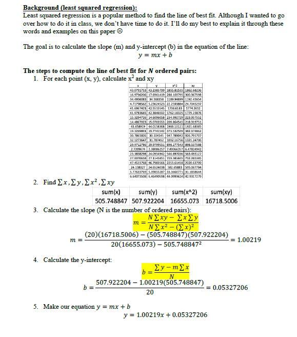
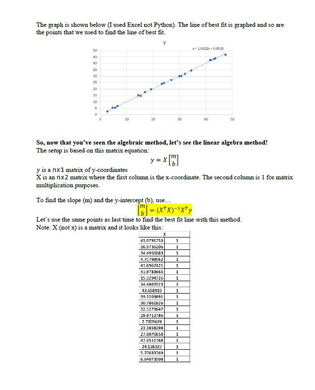
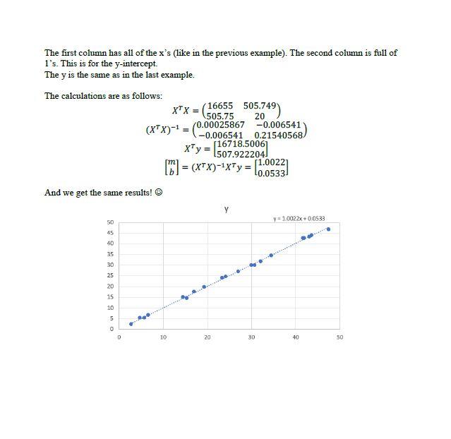
Background (least squared regression); Least squared regression is a popular method to find the line of best fit. Although I wanted to go over how to do it in class, we don't have time to do it. I'll do my best to explain it through these words and examples on this paper The goal is to calculate the slope (m) and y-intercept (b) in the equation of the line: y = mx + b The steps to compute the line of best fit for N ordered pairs: 1. For each point (x, y), calculate x and xy 2 2 43.0791753 43.2385 23335.81531362612X 169736206 17.6961419 28. 103795 390.367598 34 2956083 34568358118994699 119245654 4.717585125.2362452322 259364 24.7045297 41.0967421 42.5515545 1736103 17342612 41.0713565 12.18465922711325 172923576 15.3254726 24.6096058 234 992723 223.952552 14 4987023 15.079553 209.85454521B 319751 43.658919 4401553432906.10123 L92168385 39.3200051 29.7741542 372 53250 312.174862 10.361836 35.304945 942.3042936.799702 32.1223547 31.781452 2052.167S6 102114706 29.9722786 29.9799551898.272549 898.537588 2.7209574 2.380852ST 740356357 6.47824942 23.3958295 24.0954942546.897036563.693127 27.DODGSO 27.1145661 729.33607122851 47.6112 46.2980566 2259.68418 222061709 24.133327 246624035 582.65853 595.062784 5.77633769 5.3985528333.366673 31.338644 6.54073508 6.46490598 44 0993624 42.9317279 m = m = 2. Find Ex. 2y,3x2, Exy sum(x) sum(y) sum(x^2) sum(xy) 505.748847 507.922204 16655.073 16718.5006 3. Calculate the slope (N is the number of ordered pairs): y - ? - ()? (20)(16718.5006) - (505.748847)(507.922204) = 1.00219 20(16655.073) - 505.7488472 4. Calculate the y-intercept: Ey-mx 507.922204 - 1.00219(505.748847) 20 0.05327206 5. Make our equation y = mx + b y = 1.00219x + 0.05327206 b= The graph is shown below (I used Excel not Python). The line of best fit is graphed and so are the points that we used to find the line of best fit. y y=10022 0.0533 50 45 40 35 30 25 20 15 20 5 D 10 20 90 40 SO So, now that you've seen the algebraic method, let's see the linear algebra method! The setup is based on this matrix equation: y = x(0 y is a nx1 matrix of y-coordinates X is an nx2 matrix where the first column is the x-coordinate. The second column is 1 for matrix multiplication purposes. To find the slope (m) and the y-intercept (b), use... 101 = (x+x)-ixty Let's use the same points as last time to find the best fit line with this method. Note: X (not x) is a matrix and it looks like this: 1 1 1 1 1 X 43.0791753 16.9736205 34 4956083 4.71798562 41.6957421 41.9783665 15.3294726 14.4867023 43.658919 19.3269891 30.7851825 32.1273647 29.9712786 2.7209674 23.3858293 27.0070658 47.4511768 24.138327 5.77633769 6.64073508 1 1 1 1 1 1 1 1 1 1 1 1 1 1 1 The first column has all of the x's (like in the previous example). The second column is full of l's. This is for the y-intercept. The y is the same as in the last example. The calculations are as follows: XTX = 16655 505.749) 505.75 20 (XTX)-- = (C-00025867 -0.006541 -0.006541 0.21540568/ 507.922204 (16) = (x+X)-4x+y = [1.00221 x+y = [16718.5006 = 10.0533 And we get the same results! Y y = 1:0022x+00533 50 45 40 35 30 o 5 8 8 8 8 8 8 25 20 15 10 10 20 30 40 50 Task: 1. Take a close look at the lin_reg.py file. There are four empty functions: least_sq (file_name) and mat_least_sq (file_name) and predict (file_name, x) and plot_reg (file_name, using_matrix). Read through all of their descriptions carefully. Remember, you will lose points if you do not follow the instructions. We are using a grading script Summary of function tasks least_sq(file_name): Given the csv file_name, find the slope and y-intercept of the data using algebraic least squares (the first linear regression presented). You need to return the slope and y- intercept IN THAT ORDER. Round the slope and y-intercept to four decimal places. mat_least_sq(file_name): Given the csv file_name, find the slope and y-intercept of the data using linear algebraic least squares using matrices (the second linear regression presented). You need to return the slope and y-intercept IN THAT ORDER. Round the slope and y- intercept to four decimal places. predict(file_name, x): Given the csv file_name and an input value x, predict what the output would be using the equation that is derived from mat_least_$90. This means that you should be calling mat_least_sq in this function. Round the predicted output to four decimal places before returning the value. plot_reg(file_name, using_matrix): Given the csv file_name and an indicator of which linear regression method to use using_matrix, output a graph of the data points and the line of best fit. If using_matrix=False, then you should be plotting your results from least_sq. You should be using red for everything in the graph with X markers for the data points. If using_matrix=True, then you should be plotting your results from mat_least_sq. You can use any color but the default blue and red. You can use any data point marker except for the default dot and X. plot_reg() should not return anything. Your graphs should also contain the following: Labeled x axis Labeled y axis Graph Title Legend (see example for details) x 43.07918 43.23858 16.97362 17.69614 34.49561 34.56836 4.717986 5.236245 41.69674 42.55155 41.97837 42.38466 15.32947 14.60961 14.4867 15.07036 43.65892 44.01584 19.32699 19.77415 30.78618 30.10415 32.12736 31.78745 29.97128 29.97996 2.720967 2.380863 23.38583 24.09549 27.00707 27.11459 47.45118 46.79836 24.13833 24.6524: 5.776338 5.398553 6.640735 6.464906 Background (least squared regression); Least squared regression is a popular method to find the line of best fit. Although I wanted to go over how to do it in class, we don't have time to do it. I'll do my best to explain it through these words and examples on this paper The goal is to calculate the slope (m) and y-intercept (b) in the equation of the line: y = mx + b The steps to compute the line of best fit for N ordered pairs: 1. For each point (x, y), calculate x and xy 2 2 43.0791753 43.2385 23335.81531362612X 169736206 17.6961419 28. 103795 390.367598 34 2956083 34568358118994699 119245654 4.717585125.2362452322 259364 24.7045297 41.0967421 42.5515545 1736103 17342612 41.0713565 12.18465922711325 172923576 15.3254726 24.6096058 234 992723 223.952552 14 4987023 15.079553 209.85454521B 319751 43.658919 4401553432906.10123 L92168385 39.3200051 29.7741542 372 53250 312.174862 10.361836 35.304945 942.3042936.799702 32.1223547 31.781452 2052.167S6 102114706 29.9722786 29.9799551898.272549 898.537588 2.7209574 2.380852ST 740356357 6.47824942 23.3958295 24.0954942546.897036563.693127 27.DODGSO 27.1145661 729.33607122851 47.6112 46.2980566 2259.68418 222061709 24.133327 246624035 582.65853 595.062784 5.77633769 5.3985528333.366673 31.338644 6.54073508 6.46490598 44 0993624 42.9317279 m = m = 2. Find Ex. 2y,3x2, Exy sum(x) sum(y) sum(x^2) sum(xy) 505.748847 507.922204 16655.073 16718.5006 3. Calculate the slope (N is the number of ordered pairs): y - ? - ()? (20)(16718.5006) - (505.748847)(507.922204) = 1.00219 20(16655.073) - 505.7488472 4. Calculate the y-intercept: Ey-mx 507.922204 - 1.00219(505.748847) 20 0.05327206 5. Make our equation y = mx + b y = 1.00219x + 0.05327206 b= The graph is shown below (I used Excel not Python). The line of best fit is graphed and so are the points that we used to find the line of best fit. y y=10022 0.0533 50 45 40 35 30 25 20 15 20 5 D 10 20 90 40 SO So, now that you've seen the algebraic method, let's see the linear algebra method! The setup is based on this matrix equation: y = x(0 y is a nx1 matrix of y-coordinates X is an nx2 matrix where the first column is the x-coordinate. The second column is 1 for matrix multiplication purposes. To find the slope (m) and the y-intercept (b), use... 101 = (x+x)-ixty Let's use the same points as last time to find the best fit line with this method. Note: X (not x) is a matrix and it looks like this: 1 1 1 1 1 X 43.0791753 16.9736205 34 4956083 4.71798562 41.6957421 41.9783665 15.3294726 14.4867023 43.658919 19.3269891 30.7851825 32.1273647 29.9712786 2.7209674 23.3858293 27.0070658 47.4511768 24.138327 5.77633769 6.64073508 1 1 1 1 1 1 1 1 1 1 1 1 1 1 1 The first column has all of the x's (like in the previous example). The second column is full of l's. This is for the y-intercept. The y is the same as in the last example. The calculations are as follows: XTX = 16655 505.749) 505.75 20 (XTX)-- = (C-00025867 -0.006541 -0.006541 0.21540568/ 507.922204 (16) = (x+X)-4x+y = [1.00221 x+y = [16718.5006 = 10.0533 And we get the same results! Y y = 1:0022x+00533 50 45 40 35 30 o 5 8 8 8 8 8 8 25 20 15 10 10 20 30 40 50 Task: 1. Take a close look at the lin_reg.py file. There are four empty functions: least_sq (file_name) and mat_least_sq (file_name) and predict (file_name, x) and plot_reg (file_name, using_matrix). Read through all of their descriptions carefully. Remember, you will lose points if you do not follow the instructions. We are using a grading script Summary of function tasks least_sq(file_name): Given the csv file_name, find the slope and y-intercept of the data using algebraic least squares (the first linear regression presented). You need to return the slope and y- intercept IN THAT ORDER. Round the slope and y-intercept to four decimal places. mat_least_sq(file_name): Given the csv file_name, find the slope and y-intercept of the data using linear algebraic least squares using matrices (the second linear regression presented). You need to return the slope and y-intercept IN THAT ORDER. Round the slope and y- intercept to four decimal places. predict(file_name, x): Given the csv file_name and an input value x, predict what the output would be using the equation that is derived from mat_least_$90. This means that you should be calling mat_least_sq in this function. Round the predicted output to four decimal places before returning the value. plot_reg(file_name, using_matrix): Given the csv file_name and an indicator of which linear regression method to use using_matrix, output a graph of the data points and the line of best fit. If using_matrix=False, then you should be plotting your results from least_sq. You should be using red for everything in the graph with X markers for the data points. If using_matrix=True, then you should be plotting your results from mat_least_sq. You can use any color but the default blue and red. You can use any data point marker except for the default dot and X. plot_reg() should not return anything. Your graphs should also contain the following: Labeled x axis Labeled y axis Graph Title Legend (see example for details) x 43.07918 43.23858 16.97362 17.69614 34.49561 34.56836 4.717986 5.236245 41.69674 42.55155 41.97837 42.38466 15.32947 14.60961 14.4867 15.07036 43.65892 44.01584 19.32699 19.77415 30.78618 30.10415 32.12736 31.78745 29.97128 29.97996 2.720967 2.380863 23.38583 24.09549 27.00707 27.11459 47.45118 46.79836 24.13833 24.6524: 5.776338 5.398553 6.640735 6.464906