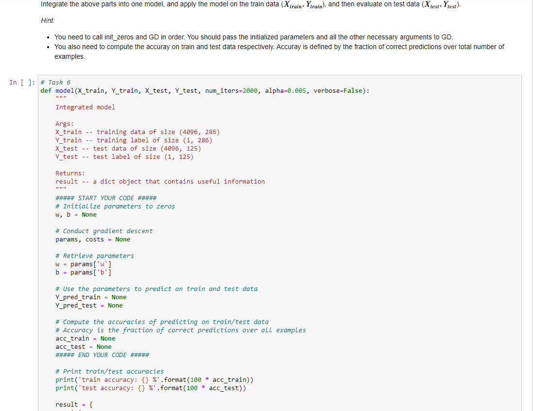
def model(X_train, Y_train, X_test, Y_test, num_iters=2000, alpha=0.005, verbose=False): """ Integrated model Args: X_train -- training data of size (4096, 286) Y_train -- training label of size (1, 286) X_test -- test data of size (4096, 125) Y_test -- test label of size (1, 125) Returns: result -- a dict object that contains useful information """ ##### START YOUR CODE ##### # Initialize parameters to zeros w, b = None # Conduct gradient descent params, costs = None # Retrieve parameters w = params['w'] b = params['b'] # Use the parameters to predict on train and test data Y_pred_train = None Y_pred_test = None # Compute the accuracies of predicting on train/test data # Accuracy is the fraction of correct predictions over all examples acc_train = None acc_test = None ##### END YOUR CODE ##### # Print train/test accuracies print('train accuracy: {} %'.format(100 * acc_train)) print('test accuracy: {} %'.format(100 * acc_test)) result = { 'w': w, 'b': b, 'costs': costs, 'Y_pred_test': Y_pred_test } return result

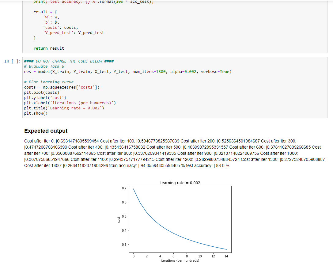
#### DO NOT CHANGE THE CODE BELOW #### # Evaluate Task 6 res = model(X_train, Y_train, X_test, Y_test, num_iters=1500, alpha=0.002, verbose=True)

# Plot learning curve costs = np.squeeze(res['costs']) plt.plot(costs) plt.ylabel('cost') plt.xlabel('iterations (per hundreds)') plt.title('Learning rate = 0.002') plt.show()

Integrate the above parts into one model, and apply the model on the train data (Xtrain,Ytrain), and then evaluate on test data (Xtest,Ytest). Hint: - You need to call init_zeros and GD in order. You should pass the initialized parameters and all the other necessary arguments to GD. - You also need to compute the accuray on train and test data respectively. Accuray is defined by the fraction of correct predictions over total number of examples. \#\#\# DO NOT CHANGE THE CODE BELOW \#\#\#\# \# Evaluate Task 6 res = model(X_train, Y_train, X_test, Y_test, num_iters=1500, alpha=0.002, verbose=True) \# Plot learning curve costs = np.squeeze(res['costs']) plt.plot(costs) plt.ylabel('cost') plt.xlabel('iterations (per hundreds)') plt.title('Learning rate =0.002 ') plt.show() Expected output Cost after iter 0: |0.6931471805599454 Cost after iter 100: |0.5946773825987639 Cost after iter 200: |0.5256364501984687 Cost after iter 300 : |0.4747208768166399 Cost after iter 400: |0.435436416758632 Cost after iter 500: |0.40399872095331557 Cost after iter 600 : |0.37811027839268685 Cost after iter 700: 0.35630887692114865 Cost after iter 800: 0.3376209341419335 Cost after iter 900:0.32137148224069756 Cost after iter 1000 : |0.30707586651947666 Cost after iter 1100: |0.29437547177794215 Cost after iter 1200: |0.28299807348845724 Cost after iter 1300: |0.27273248705908887 Cost after iter 1400: |0.26341182071904296 train accuracy: | 94.05594405594405 \% test accuracy: | 88.0%