describing data graphically and numerically

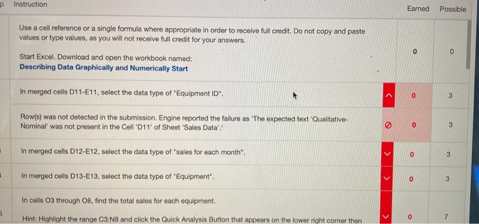
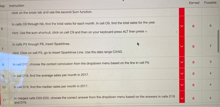
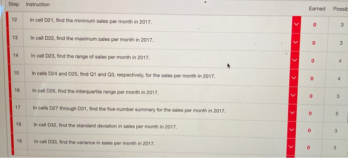
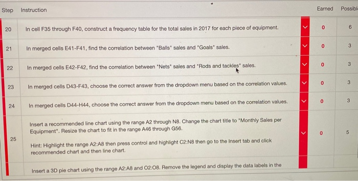
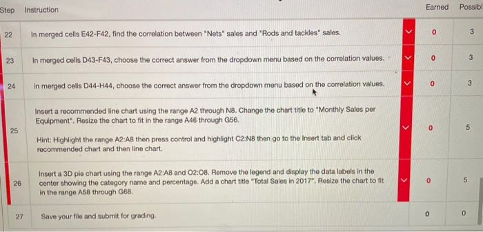
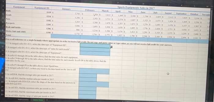
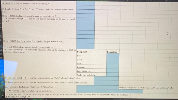
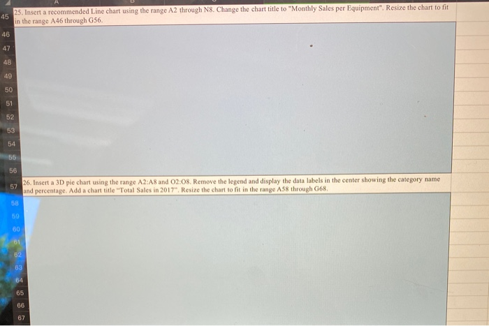
Instruction Earned Possible Use a cell reference or a single formula where appropriate in order to receive full credit. Do not copy and paste values or type values, as you will not receive full credit for your answers. Start Excel. Download and open the workbook named: Describing Data Graphically and Numerically Start 0 0 In merged cells D11-E11, select the data type of "Equipment ID". 0 3 Row(s) was not detected in the submission Engine reported the failure as 'The expected text 'Qualitative- Nominal' was not present in the Cell '011' of Sheet 'Sales Data'. 0 3 In merged cells D12-E12, select the data type of sales for each month". 0 6 6 In cells C9 through N9, find the total sales for each month. In cell 09, find the total sales for the year. Hint: Use the sum shortcut; click on cell C9 and then on your keyboard press ALT then press -. In cells P3 through P9, insert Sparklines. 7 > 0 7 Hint: Click on cell P3, go to Insert Sparklines Line. Use the data range C3:N3. 3 24 In merged cells D44-H44, choose the correct answer from the dropdown menu based on the correlation values. 0 5 o 3 24 In merged cells D44-H44, choose the correct answer from the dropdown menu based on the correlation values. 0 5 Insert a recommended line chart using the range A2 through N8. Change the chart title to "Monthly Sales por Equipment". Resize the chart to fit in the range A46 through G56. Hint: Highlight the range A2:A8 then press control and highlight C2:N8 then go to the Insert tab and click recommended chart and then line chart. 25 26 5 Insert a 3D ple chart using the range A2:A8 and 02:08. Remove the legend and display the data labels in the center showing the category name and percentage. Add a chart title "Total Sales in 2017". Resize the chart to fit in the range A58 through G68. 0 o 27 0 Save your file and submit for grading, Oktober Novem 2 1. 1.075 1 1,615 13 1 2. G 1 Sports Equipments Sales in 2017 Equipment Equipment ID February March April Mas June Jul Balls August September 1.8125 1.549 5 2.204 1.709 1895 11145 1.711S 1.5745 1,687 S 1.5715 1.045 Net 11825 1.368 1.49 1.3575 16715 1.4815 1.67% Rats 1205 103 1.670 1.776 1915 155 Rod and tackle 12065 8865 214 1945 1.2913 15 Sticks, bars and clubs 1145 1,712 1.161 1.773 1. 200 20 S 2056 Total Use a cell referencer a single formula where appropriate in der to refullt. Dessertype values, syee will tree full credit for your 1-2. In merge cells DII-11 lect the datatype of "ID 1.In menged cells 12-12, select the date type of each month In merged cells 14). Select the data type of "Equipment 44 5.In cells through Os in the bove, elles for each In cells through N9 in the table shove, find the total sales for each month in all is the the show, find the otal sales for the year 2. In cells through in the table above, insert Sparklines Ismered cells 17-19. Is there any trend in the data based on the line in cell P9 4 In cel DI find the average sales per month in 2017 10. In cell D1%, find the media sales per month in 2017 20 11. Is merged cells 030-20, select the shape of the data based on the wes is Dell Dixind DIS 12 is cell 021.fed the minimum sales person in 2011 22 11 locall fod the maximum sales month in 2017 23 s cell the range of sales per month 2017 ructor Sales Data 14. In cell D23, find the range of sales per month in 2017 IS. In cells D24 and D25, find Q1 and 03, respectively, for the sales per month in 2017 16. In cell D26, find the interquartile range per month in 2017. 17. In cells D27 through D31, find the five-number summary for the sales per month in 2017 + 1 Percentage 2 18. In cell D32, find the standard deviation in sales per month in 2017 13 19. In cell D33, find the variance in sales per month in 2017. 34 20. In cell P35 through F40, construct a frequency table for the total sales in 2017 for cach piece of equipment Equipment 35 Balls 38 Goals Nets Racquets Rods and tackle Sticks, bars and clubs 41 21. In merged cells E41.741, find the correlation between "Balls sales and "Goals sales. 42 22. In merged cells E42.742, find the correlation between "Nets" sales and Rods and tackle sales 43 23. The relationship between Balls sales & Goals sales is the relationship between "Nets" sales and "Rods and tackle ules 44 24. Based on the correlation values, we can conlude that 45 25. Insert a recommended Line chart using the range A2 through N. Change the chart title to "Monthly sales per Equipment Resize the chart to fit in the range Alb through 656 SD India 45 25. Insert a recommended Line chart using the range A2 through N8. Change the chart title to "Monthly Sales per Equipment". Resize the chart to fit in the range A46 through G56. 46 48 49 50 51 52 53 54 56 56 57 26. Insert a 3D pie chart using the range A2:A8 and 02:08. Remove the legend and display the data labels in the center showing the category name and percentage. Add a chart title "Total Sales in 2017". Resize the chart to fit in the range A58 through G68 58 50 60 61 62 63 64 65 66 67 Exent Total Ralli FRID 11195 11145 1.18 1945 13 S 1,2635 TIKS 1206 April May A 1,7995 195 1595 1.5235 13735 1,4995 1,275 5 1938 1,670 1.895.5 US 1.45 LINS 1.291 BAS 1.200 Sraber 21125 14245 1 16785 1.157 11S 18565 1373 S 1.2555 2,465 NoDesember 3514 5 2,414 ISMS 2,150 15075 1615 16715 1.9075 1,994 1.455 1.400 5 1.54 2,1615 2.542 Is Red and tackle 135 $19 1125S 1,7613 Instruction Earned Possible Use a cell reference or a single formula where appropriate in order to receive full credit. Do not copy and paste values or type values, as you will not receive full credit for your answers. Start Excel. Download and open the workbook named: Describing Data Graphically and Numerically Start 0 0 In merged cells D11-E11, select the data type of "Equipment ID". 0 3 Row(s) was not detected in the submission Engine reported the failure as 'The expected text 'Qualitative- Nominal' was not present in the Cell '011' of Sheet 'Sales Data'. 0 3 In merged cells D12-E12, select the data type of sales for each month". 0 6 6 In cells C9 through N9, find the total sales for each month. In cell 09, find the total sales for the year. Hint: Use the sum shortcut; click on cell C9 and then on your keyboard press ALT then press -. In cells P3 through P9, insert Sparklines. 7 > 0 7 Hint: Click on cell P3, go to Insert Sparklines Line. Use the data range C3:N3. 3 24 In merged cells D44-H44, choose the correct answer from the dropdown menu based on the correlation values. 0 5 o 3 24 In merged cells D44-H44, choose the correct answer from the dropdown menu based on the correlation values. 0 5 Insert a recommended line chart using the range A2 through N8. Change the chart title to "Monthly Sales por Equipment". Resize the chart to fit in the range A46 through G56. Hint: Highlight the range A2:A8 then press control and highlight C2:N8 then go to the Insert tab and click recommended chart and then line chart. 25 26 5 Insert a 3D ple chart using the range A2:A8 and 02:08. Remove the legend and display the data labels in the center showing the category name and percentage. Add a chart title "Total Sales in 2017". Resize the chart to fit in the range A58 through G68. 0 o 27 0 Save your file and submit for grading, Oktober Novem 2 1. 1.075 1 1,615 13 1 2. G 1 Sports Equipments Sales in 2017 Equipment Equipment ID February March April Mas June Jul Balls August September 1.8125 1.549 5 2.204 1.709 1895 11145 1.711S 1.5745 1,687 S 1.5715 1.045 Net 11825 1.368 1.49 1.3575 16715 1.4815 1.67% Rats 1205 103 1.670 1.776 1915 155 Rod and tackle 12065 8865 214 1945 1.2913 15 Sticks, bars and clubs 1145 1,712 1.161 1.773 1. 200 20 S 2056 Total Use a cell referencer a single formula where appropriate in der to refullt. Dessertype values, syee will tree full credit for your 1-2. In merge cells DII-11 lect the datatype of "ID 1.In menged cells 12-12, select the date type of each month In merged cells 14). Select the data type of "Equipment 44 5.In cells through Os in the bove, elles for each In cells through N9 in the table shove, find the total sales for each month in all is the the show, find the otal sales for the year 2. In cells through in the table above, insert Sparklines Ismered cells 17-19. Is there any trend in the data based on the line in cell P9 4 In cel DI find the average sales per month in 2017 10. In cell D1%, find the media sales per month in 2017 20 11. Is merged cells 030-20, select the shape of the data based on the wes is Dell Dixind DIS 12 is cell 021.fed the minimum sales person in 2011 22 11 locall fod the maximum sales month in 2017 23 s cell the range of sales per month 2017 ructor Sales Data 14. In cell D23, find the range of sales per month in 2017 IS. In cells D24 and D25, find Q1 and 03, respectively, for the sales per month in 2017 16. In cell D26, find the interquartile range per month in 2017. 17. In cells D27 through D31, find the five-number summary for the sales per month in 2017 + 1 Percentage 2 18. In cell D32, find the standard deviation in sales per month in 2017 13 19. In cell D33, find the variance in sales per month in 2017. 34 20. In cell P35 through F40, construct a frequency table for the total sales in 2017 for cach piece of equipment Equipment 35 Balls 38 Goals Nets Racquets Rods and tackle Sticks, bars and clubs 41 21. In merged cells E41.741, find the correlation between "Balls sales and "Goals sales. 42 22. In merged cells E42.742, find the correlation between "Nets" sales and Rods and tackle sales 43 23. The relationship between Balls sales & Goals sales is the relationship between "Nets" sales and "Rods and tackle ules 44 24. Based on the correlation values, we can conlude that 45 25. Insert a recommended Line chart using the range A2 through N. Change the chart title to "Monthly sales per Equipment Resize the chart to fit in the range Alb through 656 SD India 45 25. Insert a recommended Line chart using the range A2 through N8. Change the chart title to "Monthly Sales per Equipment". Resize the chart to fit in the range A46 through G56. 46 48 49 50 51 52 53 54 56 56 57 26. Insert a 3D pie chart using the range A2:A8 and 02:08. Remove the legend and display the data labels in the center showing the category name and percentage. Add a chart title "Total Sales in 2017". Resize the chart to fit in the range A58 through G68 58 50 60 61 62 63 64 65 66 67 Exent Total Ralli FRID 11195 11145 1.18 1945 13 S 1,2635 TIKS 1206 April May A 1,7995 195 1595 1.5235 13735 1,4995 1,275 5 1938 1,670 1.895.5 US 1.45 LINS 1.291 BAS 1.200 Sraber 21125 14245 1 16785 1.157 11S 18565 1373 S 1.2555 2,465 NoDesember 3514 5 2,414 ISMS 2,150 15075 1615 16715 1.9075 1,994 1.455 1.400 5 1.54 2,1615 2.542 Is Red and tackle 135 $19 1125S 1,7613
