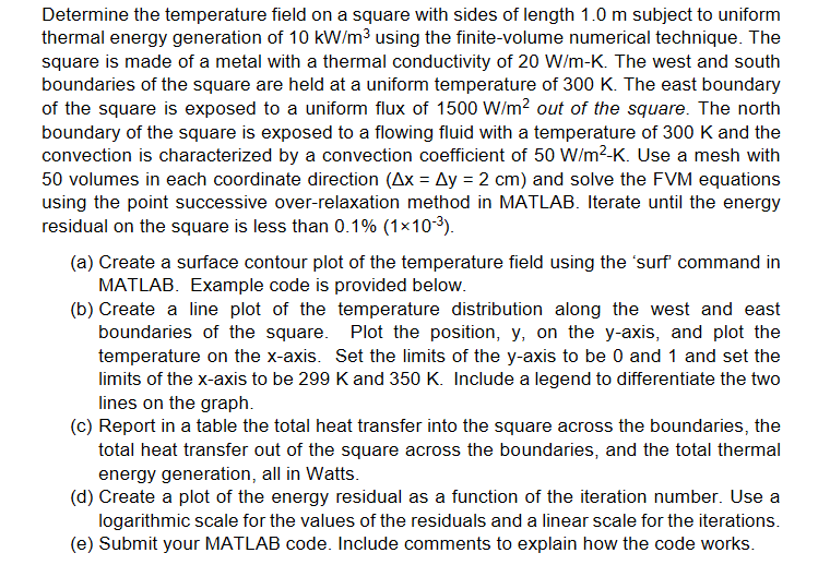
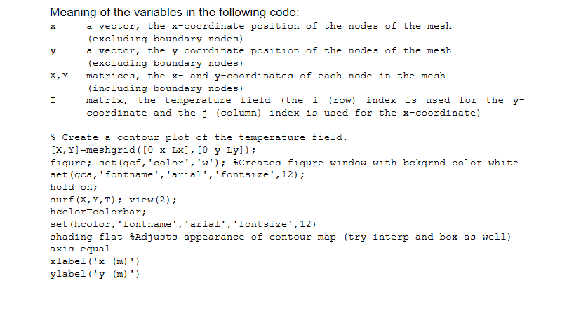
Determine the temperature field on a square with sides of length 1.0 m subject to uniform thermal energy generation of 10 kW/m3 using the finite-volume numerical technique. The square is made of a metal with a thermal conductivity of 20 W/m-K. The west and south boundaries of the square are held at a uniform temperature of 300 K. The east boundary of the square is exposed to a uniform flux of 1500 W/m2 out of the square. The north boundary of the square is exposed to a flowing fluid with a temperature of 300 K and the convection is characterized by a convection coefficient of 50 W/mK. Use a mesh with 50 volumes in each coordinate direction (Ax = Ay = 2 cm) and solve the FVM equations using the point successive over-relaxation method in MATLAB. Iterate until the energy residual on the square is less than 0.1% (1x103). (a) Create a surface contour plot of the temperature field using the 'surf command in MATLAB. Example code is provided below. (b) Create a line plot of the temperature distribution along the west and east boundaries of the square. Plot the position, y, on the y-axis, and plot the temperature on the x-axis. Set the limits of the y-axis to be 0 and 1 and set the limits of the x-axis to be 299 K and 350 K. Include a legend to differentiate the two lines on the graph. (c) Report in a table the total heat transfer into the square across the boundaries, the total heat transfer out of the square across the boundaries, and the total thermal energy generation, all in Watts. (d) Create a plot of the energy residual as a function of the iteration number. Use a logarithmic scale for the values of the residuals and a linear scale for the iterations. (e) Submit your MATLAB code. Include comments to explain how the code works. Y Meaning of the variables in the following code: a vector, the x-coordinate position of the nodes of the mesh (excluding boundary nodes) a vector, the y-coordinate position of the nodes of the mesh (excluding boundary nodes) X, Y matrices, the x- and y-coordinates of each node in the mesh (including boundary nodes) matrix, the temperature field (the i (row) index for the y- coordinate and the j (column) index is used for the x-coordinate) T is used Create a contour plot of the temperature field. [X,Y)=meshgrid([0 x Lx], [0 y Ly]); figure; set (gcf, 'color', 'w'); $Creates figure windo with bckgrnd co te set (gca,'fontname','arial','fontsize', 12); hold on; surf (X, Y,T); view (2); hcolor=colorbar; set (hcolor, 'fontname', 'arial','fontsize', 12) shading flat Adjusts appearance of contour map (try interp and box as well) axis equal xlabel('x (m)') ylabel('y (m)') Determine the temperature field on a square with sides of length 1.0 m subject to uniform thermal energy generation of 10 kW/m3 using the finite-volume numerical technique. The square is made of a metal with a thermal conductivity of 20 W/m-K. The west and south boundaries of the square are held at a uniform temperature of 300 K. The east boundary of the square is exposed to a uniform flux of 1500 W/m2 out of the square. The north boundary of the square is exposed to a flowing fluid with a temperature of 300 K and the convection is characterized by a convection coefficient of 50 W/mK. Use a mesh with 50 volumes in each coordinate direction (Ax = Ay = 2 cm) and solve the FVM equations using the point successive over-relaxation method in MATLAB. Iterate until the energy residual on the square is less than 0.1% (1x103). (a) Create a surface contour plot of the temperature field using the 'surf command in MATLAB. Example code is provided below. (b) Create a line plot of the temperature distribution along the west and east boundaries of the square. Plot the position, y, on the y-axis, and plot the temperature on the x-axis. Set the limits of the y-axis to be 0 and 1 and set the limits of the x-axis to be 299 K and 350 K. Include a legend to differentiate the two lines on the graph. (c) Report in a table the total heat transfer into the square across the boundaries, the total heat transfer out of the square across the boundaries, and the total thermal energy generation, all in Watts. (d) Create a plot of the energy residual as a function of the iteration number. Use a logarithmic scale for the values of the residuals and a linear scale for the iterations. (e) Submit your MATLAB code. Include comments to explain how the code works. Y Meaning of the variables in the following code: a vector, the x-coordinate position of the nodes of the mesh (excluding boundary nodes) a vector, the y-coordinate position of the nodes of the mesh (excluding boundary nodes) X, Y matrices, the x- and y-coordinates of each node in the mesh (including boundary nodes) matrix, the temperature field (the i (row) index for the y- coordinate and the j (column) index is used for the x-coordinate) T is used Create a contour plot of the temperature field. [X,Y)=meshgrid([0 x Lx], [0 y Ly]); figure; set (gcf, 'color', 'w'); $Creates figure windo with bckgrnd co te set (gca,'fontname','arial','fontsize', 12); hold on; surf (X, Y,T); view (2); hcolor=colorbar; set (hcolor, 'fontname', 'arial','fontsize', 12) shading flat Adjusts appearance of contour map (try interp and box as well) axis equal xlabel('x (m)') ylabel('y (m)')