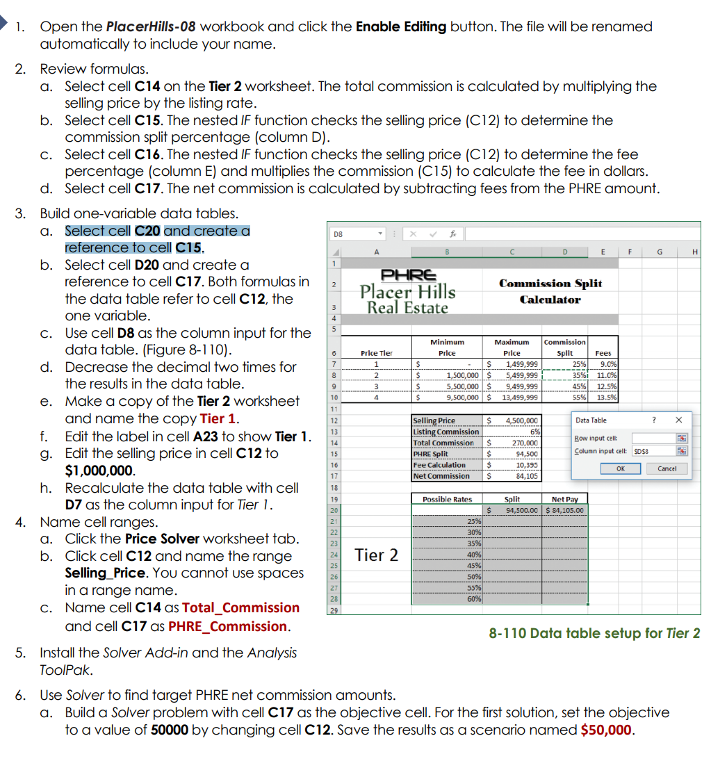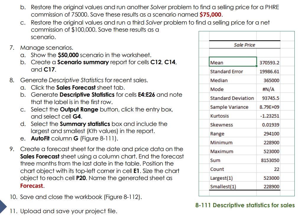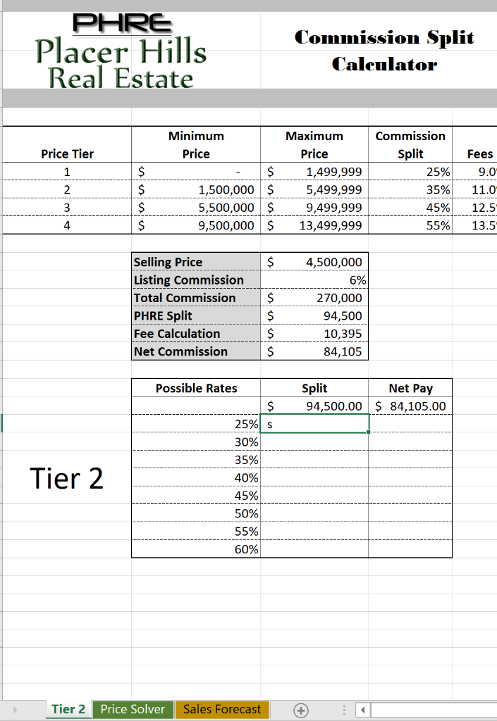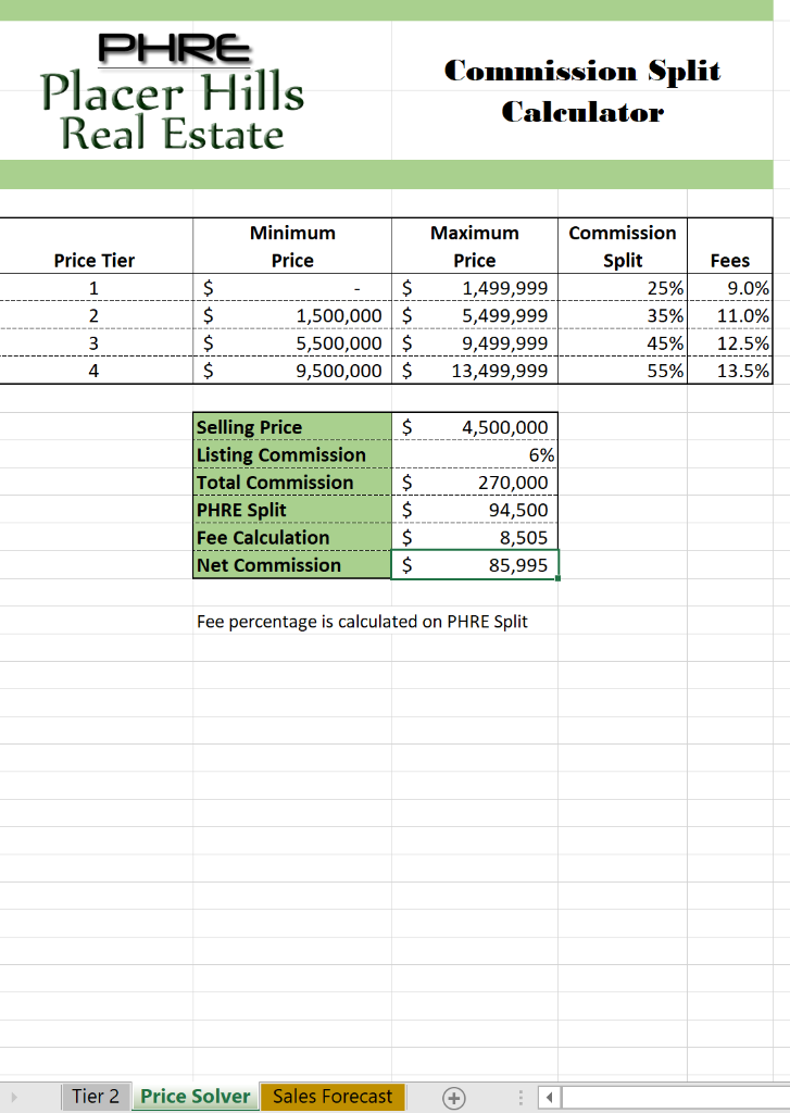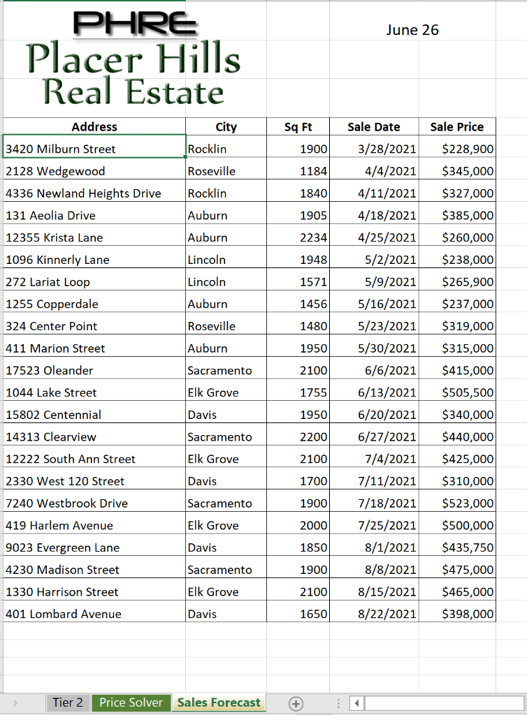
DS E F G H 1. Open the placerHills-08 workbook and click the Enable Editing button. The file will be renamed automatically to include your name. 2. Review formulas. a. Select cell C14 on the Tier 2 worksheet. The total commission is calculated by multiplying the selling price by the listing rate. b. Select cell C15. The nested IF function checks the selling price (C12) to determine the commission split percentage (column D). C. Select cell C16. The nested IF function checks the selling price (C12) to determine the fee percentage (column E) and multiplies the commission (C15) to calculate the fee in dollars. d. Select cell C17. The net commission is calculated by subtracting fees from the PHRE amount. 3. Build one-variable data tables. a. Select cell C20 and create a reference to cell C15. AD b. Select cell D20 and create a reference to cell C17. Both formulas in PHRE Commission Split the data table refer to cell C12, the Placer Hills Calculator Real Estate one variable. c. Use cell D8 as the column input for the Commission data table. (Figure 8-110). d. Decrease the decimal two times for 25% 8 35% the results in the data table. 45% e. Make a copy of the Tier 2 worksheet and name the copy Tier 1. Selling Price 4,500,000 f. 6% Edit the label in cell A23 to show Tier 1. Listing Commission 270,000 g. Edit the selling price in cell C12 to Fee Calculation $1,000,000. h. Recalculate the data table with cell D7 as the column input for Tier 1. 20 4. Name cell ranges. 25% 30% a. Click the Price Solver worksheet tab. 35% b. Click cell C12 and name the range Tier 2 40% Selling Price. You cannot use spaces in a range name. c. Name cell C14 as Total_Commission and cell C17 as PHRE_Commission. 8-110 Data table setup for Tier 2 5. Install the Solver Add-in and the Analysis ToolPak. Minimum Price Split 6 7 Price Tier 1 2 3 3 4 $ $ S 3 $ Maximum Price $ 1,499,999 $ 5,499,999 $ 9,499,999 $ 13,499,999 1,500,000 5,500,000 9,500,000 Fees 9.0% 11.09 12.5% 13.596 10 55% 11 1 $ Data Table ? 12 13 14 15 16 10 17 1 10 18 Total Commission PHRE Split Row input cell Column input cell: SD$8 ES $ $ $ $ 94,500 10,395 84,105 OK Cancel Net Commission 19 Possible Rates Split 94,500.00 Net Pay $ 84,105.00 $ 2 45% 5096 55% 60% 6. Use Solver to find target PHRE net commission amounts. a. Build a Solver problem with cell C17 as the objective cell. For the first solution, set the objective to a value of 50000 by changing cell C12. Save the results as a scenario named $50,000. b. Restore the original values and run another Solver problem to find a selling price for a PHRE commission of 75000. Save these results as a scenario named $75,000. c. Restore the original values and run a third Solver problem to find a selling price for a net commission of $100,000. Save these results as a scenario. Sale Price 7. Manage scenarios. a. Show the $50,000 scenario in the worksheet. b. Create a Scenario summary report for cells C12, C14, Mean 370593.2 and C17. Standard Error 19986.61 8. Generate Descriptive Statistics for recent sales. Median 365000 a. Click the Sales Forecast sheet tab. Mode #N/A b. Generate Descriptive Statistics for cells E4:E26 and note Standard Deviation 93745.5 that the label is in the first row. 8.79E+09 C. Select the Output Range button, click the entry box, Sample Variance and select cell G4. Kurtosis -1.23251 d. Select the Summary statistics box and include the Skewness 0.01939 largest and smallest (Kth values) in the report. Range 294100 e. AutoFit column G (Figure 8-111). Minimum 228900 9. Create a forecast sheet for the date and price data on the Maximum 523000 Sales Forecast sheet using a column chart. End the forecast Sum 8153050 three months from the last date in the table. Position the chart object with its top-left corner in cell E1. Size the chart Count 22 object to reach cell P20. Name the generated sheet as Largest(1) 523000 Forecast Smallest(1) 228900 10. Save and close the workbook (Figure 8-112). 8-111 Descriptive statistics for sales 11. Upload and save your project file. PHRE Placer Hills Real Estate Commission Split Calculator Price Tier 1 Minimum Price $ 1,500,000 $ 5,500,000 $ 9,500,000 $ Maximum Price 1,499,999 5,499,999 9,499,999 13,499,999 Commission Split 25% 35% $ $ $ $ 2 Fees 9.0 11.0 12.5 13.5 3 45% 4 55% $ Selling Price Listing Commission Total Commission PHRE Split Fee Calculation Net Commission $ $ $ $ 4,500,000 6% 270,000 94,500 10,395 84,105 Net Pay Split 94,500.00 $ 84,105.00 Tier 2 Possible Rates $ 25% s 30% 35% 40% 45% 50% 55% 60% Tier 2 Price Solver Sales Forecast PHRE Placer Hills Real Estate Commission Split Calculator Price Tier 1 Minimum Price $ 1,500,000 $ 5,500,000 $ 9,500,000 $ $ $ $ $ Maximum Price 1,499,999 5,499,999 9,499,999 13,499,999 Commission Split 25% 35% 45% 55% 2 Fees 9.0% 11.0% 12.5% 13.5% 3 4 $ Selling Price Listing Commission Total Commission PHRE Split Fee Calculation Net Commission $ $ $ $ 4,500,000 6% 270,000 94,500 8,505 85,995 Fee percentage is calculated on PHRE Split Tier 2 Price Solver Sales Forecast + June 26 PHRE Placer Hills Real Estate Address City Sq Ft Sale Date Sale Price 3420 Milburn Street Rocklin 1900 Roseville 1184 2128 Wedgewood 4336 Newland Heights Drive Rocklin 1840 131 Aeolia Drive Auburn 1905 3/28/2021 4/4/2021 4/11/2021 4/18/2021 4/25/2021 5/2/2021 5/9/2021 12355 Krista Lane Auburn 2234 1096 Kinnerly Lane Lincoln 1948 $228,900 $345,000 $327,000 $385,000 $260,000 $238,000 $265,900 $237,000 $319,000 $315,000 $415,000 $505,500 272 Lariat Loop Lincoln 1571 1255 Copperdale Auburn 1456 324 Center Point Roseville 1480 411 Marion Street Auburn 1950 17523 Oleander Sacramento 2100 1044 Lake Street Elk Grove 1755 15802 Centennial Davis 1950 $340,000 14313 Clearview Sacramento 2200 12222 South Ann Street Elk Grove 2100 5/16/2021 5/23/2021 5/30/2021 6/6/2021 6/13/2021 6/20/2021 6/27/2021 7/4/2021 7/11/2021 7/18/2021 7/25/2021 8/1/2021 8/8/2021 8/15/2021 8/22/2021 2330 West 120 Street Davis 1700 7240 Westbrook Drive Sacramento 1900 419 Harlem Avenue Elk Grove 2000 $440,000 $425,000 $310,000 $523,000 $500,000 $435,750 $475,000 $465,000 $398,000 9023 Evergreen Lane Davis 1850 4230 Madison Street Sacramento 1900 1330 Harrison Street Elk Grove 2100 401 Lombard Avenue Davis 1650 Tier 2 Price Solver Sales Forecast + DS E F G H 1. Open the placerHills-08 workbook and click the Enable Editing button. The file will be renamed automatically to include your name. 2. Review formulas. a. Select cell C14 on the Tier 2 worksheet. The total commission is calculated by multiplying the selling price by the listing rate. b. Select cell C15. The nested IF function checks the selling price (C12) to determine the commission split percentage (column D). C. Select cell C16. The nested IF function checks the selling price (C12) to determine the fee percentage (column E) and multiplies the commission (C15) to calculate the fee in dollars. d. Select cell C17. The net commission is calculated by subtracting fees from the PHRE amount. 3. Build one-variable data tables. a. Select cell C20 and create a reference to cell C15. AD b. Select cell D20 and create a reference to cell C17. Both formulas in PHRE Commission Split the data table refer to cell C12, the Placer Hills Calculator Real Estate one variable. c. Use cell D8 as the column input for the Commission data table. (Figure 8-110). d. Decrease the decimal two times for 25% 8 35% the results in the data table. 45% e. Make a copy of the Tier 2 worksheet and name the copy Tier 1. Selling Price 4,500,000 f. 6% Edit the label in cell A23 to show Tier 1. Listing Commission 270,000 g. Edit the selling price in cell C12 to Fee Calculation $1,000,000. h. Recalculate the data table with cell D7 as the column input for Tier 1. 20 4. Name cell ranges. 25% 30% a. Click the Price Solver worksheet tab. 35% b. Click cell C12 and name the range Tier 2 40% Selling Price. You cannot use spaces in a range name. c. Name cell C14 as Total_Commission and cell C17 as PHRE_Commission. 8-110 Data table setup for Tier 2 5. Install the Solver Add-in and the Analysis ToolPak. Minimum Price Split 6 7 Price Tier 1 2 3 3 4 $ $ S 3 $ Maximum Price $ 1,499,999 $ 5,499,999 $ 9,499,999 $ 13,499,999 1,500,000 5,500,000 9,500,000 Fees 9.0% 11.09 12.5% 13.596 10 55% 11 1 $ Data Table ? 12 13 14 15 16 10 17 1 10 18 Total Commission PHRE Split Row input cell Column input cell: SD$8 ES $ $ $ $ 94,500 10,395 84,105 OK Cancel Net Commission 19 Possible Rates Split 94,500.00 Net Pay $ 84,105.00 $ 2 45% 5096 55% 60% 6. Use Solver to find target PHRE net commission amounts. a. Build a Solver problem with cell C17 as the objective cell. For the first solution, set the objective to a value of 50000 by changing cell C12. Save the results as a scenario named $50,000. b. Restore the original values and run another Solver problem to find a selling price for a PHRE commission of 75000. Save these results as a scenario named $75,000. c. Restore the original values and run a third Solver problem to find a selling price for a net commission of $100,000. Save these results as a scenario. Sale Price 7. Manage scenarios. a. Show the $50,000 scenario in the worksheet. b. Create a Scenario summary report for cells C12, C14, Mean 370593.2 and C17. Standard Error 19986.61 8. Generate Descriptive Statistics for recent sales. Median 365000 a. Click the Sales Forecast sheet tab. Mode #N/A b. Generate Descriptive Statistics for cells E4:E26 and note Standard Deviation 93745.5 that the label is in the first row. 8.79E+09 C. Select the Output Range button, click the entry box, Sample Variance and select cell G4. Kurtosis -1.23251 d. Select the Summary statistics box and include the Skewness 0.01939 largest and smallest (Kth values) in the report. Range 294100 e. AutoFit column G (Figure 8-111). Minimum 228900 9. Create a forecast sheet for the date and price data on the Maximum 523000 Sales Forecast sheet using a column chart. End the forecast Sum 8153050 three months from the last date in the table. Position the chart object with its top-left corner in cell E1. Size the chart Count 22 object to reach cell P20. Name the generated sheet as Largest(1) 523000 Forecast Smallest(1) 228900 10. Save and close the workbook (Figure 8-112). 8-111 Descriptive statistics for sales 11. Upload and save your project file. PHRE Placer Hills Real Estate Commission Split Calculator Price Tier 1 Minimum Price $ 1,500,000 $ 5,500,000 $ 9,500,000 $ Maximum Price 1,499,999 5,499,999 9,499,999 13,499,999 Commission Split 25% 35% $ $ $ $ 2 Fees 9.0 11.0 12.5 13.5 3 45% 4 55% $ Selling Price Listing Commission Total Commission PHRE Split Fee Calculation Net Commission $ $ $ $ 4,500,000 6% 270,000 94,500 10,395 84,105 Net Pay Split 94,500.00 $ 84,105.00 Tier 2 Possible Rates $ 25% s 30% 35% 40% 45% 50% 55% 60% Tier 2 Price Solver Sales Forecast PHRE Placer Hills Real Estate Commission Split Calculator Price Tier 1 Minimum Price $ 1,500,000 $ 5,500,000 $ 9,500,000 $ $ $ $ $ Maximum Price 1,499,999 5,499,999 9,499,999 13,499,999 Commission Split 25% 35% 45% 55% 2 Fees 9.0% 11.0% 12.5% 13.5% 3 4 $ Selling Price Listing Commission Total Commission PHRE Split Fee Calculation Net Commission $ $ $ $ 4,500,000 6% 270,000 94,500 8,505 85,995 Fee percentage is calculated on PHRE Split Tier 2 Price Solver Sales Forecast + June 26 PHRE Placer Hills Real Estate Address City Sq Ft Sale Date Sale Price 3420 Milburn Street Rocklin 1900 Roseville 1184 2128 Wedgewood 4336 Newland Heights Drive Rocklin 1840 131 Aeolia Drive Auburn 1905 3/28/2021 4/4/2021 4/11/2021 4/18/2021 4/25/2021 5/2/2021 5/9/2021 12355 Krista Lane Auburn 2234 1096 Kinnerly Lane Lincoln 1948 $228,900 $345,000 $327,000 $385,000 $260,000 $238,000 $265,900 $237,000 $319,000 $315,000 $415,000 $505,500 272 Lariat Loop Lincoln 1571 1255 Copperdale Auburn 1456 324 Center Point Roseville 1480 411 Marion Street Auburn 1950 17523 Oleander Sacramento 2100 1044 Lake Street Elk Grove 1755 15802 Centennial Davis 1950 $340,000 14313 Clearview Sacramento 2200 12222 South Ann Street Elk Grove 2100 5/16/2021 5/23/2021 5/30/2021 6/6/2021 6/13/2021 6/20/2021 6/27/2021 7/4/2021 7/11/2021 7/18/2021 7/25/2021 8/1/2021 8/8/2021 8/15/2021 8/22/2021 2330 West 120 Street Davis 1700 7240 Westbrook Drive Sacramento 1900 419 Harlem Avenue Elk Grove 2000 $440,000 $425,000 $310,000 $523,000 $500,000 $435,750 $475,000 $465,000 $398,000 9023 Evergreen Lane Davis 1850 4230 Madison Street Sacramento 1900 1330 Harrison Street Elk Grove 2100 401 Lombard Avenue Davis 1650 Tier 2 Price Solver Sales Forecast +