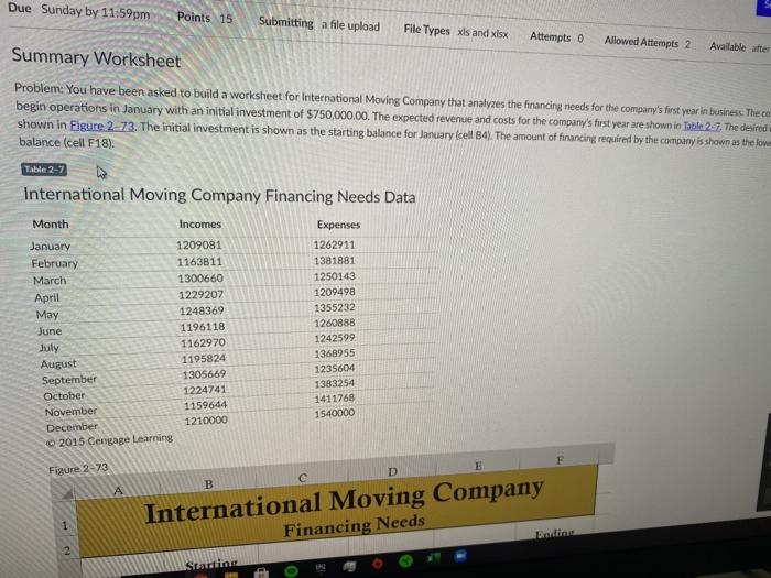
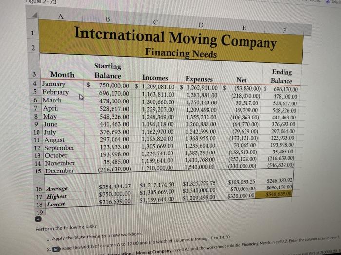
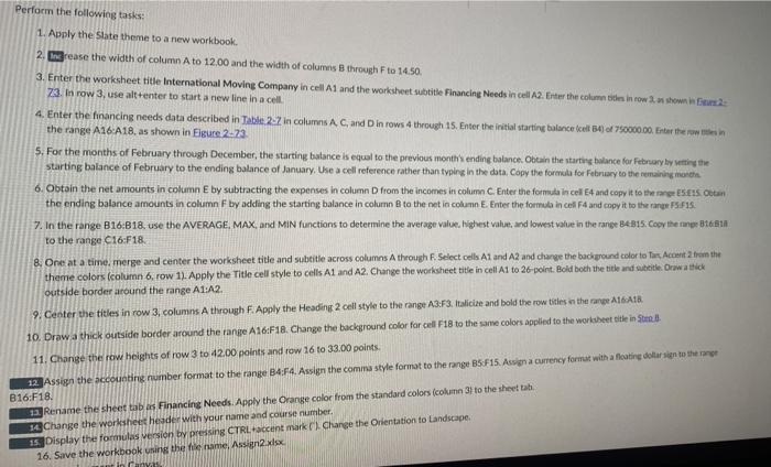
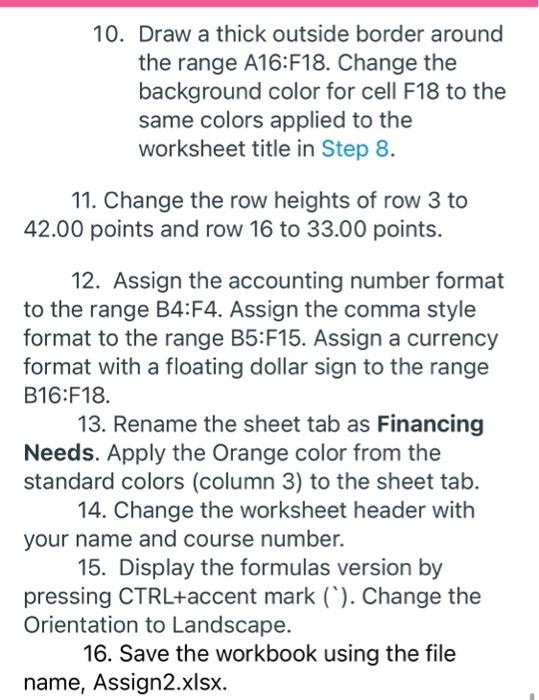
Due Sunday by 11:59pm Points 15 Submitting a file upload File Types xls and xlsx Allowed Attempts 2 Available after Attempts 0 Summary Worksheet Problem: You have been asked to build a worksheet for International Moving Company that analyzes the financing needs for the company's first year in business. The ca begin operations in January with an initial investment of $750,000.00. The expected revenue and costs for the company's first year are shown in Table 2-7. The desired shown in Figure 2-73. The initial investment is shown as the starting balance for January (cell B4). The amount of financing required by the company is shown as the low balance (cell F18) Table 27 International Moving Company Financing Needs Data Month Incomes Expenses January 1209081 1262911 February 1163811 1381881 March 1300660 1250143 April 1229207 1209498 May 1248369 1355232 June 1196118 1260888 July 1162970 1242599 1195824 1368955 August 1305669 1235604 September 1383254 October 1224741 1411768 1159644 November 1540000 December 1210000 2015 Cengage Learning D Figure 2-73 E B A 1 International Moving Company Financing Needs Erode Starting 2-73 A B @ D E F 1 2 International Moving Company Financing Needs Starting 3 Month 4 January 5 February 6 March 7 April 8 May 9 June 10 July 11 August 12 September 13 October 14 November 15 December Balance Ending Incomes Expenses Net Balance $ 750,000.00 $ 1,209,081,00 $ 1,262,911.00 $ (53,830.00) $696,170.00 696,170.00 1,163,811.00 1,381,881.00 (218,070.00) 478,100.00 478,100.00 1,300,660.00 1,250,143.00 50,517.00 528,617.00 528,617.00 1,229,207.00 1,209,498.00 19.709.00 548,326.00 548,326.00 1,248,369.00 1,355,232.00 (106,863.00) 441,463.00 441,463.00 1,196,118.00 1,260,888.00 (64,770.00) 376,693.00 376,693.00 1,162,970.00 1,242,599.00 (19,629.00) 297,064.00 297,064.00 1,195,824.00 1,368,955.00 (173,131.00) 123,933.00 123,933.00 1,305,669.00 1.235,604.00 70,065,00 193,998.00 193,998.00 1,224,741.00 1,383,254.00 35,485.00 (158,513.00) 35,485.00 1,159,614.00 1.411.768.00 (252,124.00) (216,639.00) 1,210,000.00 (216,639.00) 1,540,000.00 (330,000.00) (546,639.00) $354.434.17 $750,000.00 $216,639.00 $1.325,227.75 S1,510,000.00 $1.209.498.00 $1,217.174.50 $1,305,669.00 $1,159,614.00 $108,053.25 $70,065.00 $330,000.00 16 Average 17 Highest 18 Lowest 19 + $246,380.92 $696,170.00 $546,639.00 Perform the following tasks: 1. Apply the State theme to a new workbook 2. Increase the width of column A to 12.00 and the width of columns B through F to 14.50. mational Moving Company in cel A1 and the worksheet subtitle Financing Needs in cel A2 Enter the cities in row her Perform the following tasks: 1. Apply the Slate theme to a new workbook. 2. Ingrease the width of column A to 12.00 and the width of columns through Fto 14.50. 3. Enter the worksheet title International Moving Company in cell A1 and the worksheet subtitle Financing Needs in cel A2. Enter the columnes in rows shown in 2 23. In row 3, use alt+enter to start a new line in a cell 4. Enter the financing needs data described in Table 22 in columns AC and Din rows 4 through 15. Enter the initial starting balance cell 4 of 750000.00. Enter the we the range A16:A18, as shown in Figure 2-23 5. For the months of February through December, the starting balance is equal to the previous month's ending balance. Obtain the starting balance for February hy wetting the Starting balance of February to the ending balance of January. Use a cell reference rather than typing in the data. Copy the formula for February to the remaining nende 6. Obtain the net amounts in column E by subtracting the expenses in columnD from the incomes in column C. Enter the formula in cel E4 and copy it to the agrees ootan the ending balance amounts in column F boy adeling the starting balance in column B to the net in column E Enter the formula in cell F4 and copy it to the range E5515. 7. In the range B16:818. use the AVERAGE. MAX, and MIN functions to determine the average value Highest value and lowest value in the range B&Bs.Coy the top 316811 to the range C16:F18 8. One at a time, merge and center the worksheet title and subtitle across columns A through F. Select cells A1 and A2 and change the background color to Tax Accent theme colors (column 6. row 1). Apply the Title cell style to cells A1 and A2. Change the worksheet title in cell A1 to 26-point. Bold both the title and title Draw a thick outside border around the range A1:A2. 9. Center the titles in row 3 columns A through F. Apply the Heading 2 cell style to the range A3:F3. Italicize and bold the row titles in the range A16A1B. 10. Draw a thick outside border around the range A16:18. Change the background color for cell F18 to the same colors applied to the worksheet title in Stut. 11. Change the row heights of row 3 to 42.00 points and row 16 to 33.00 points 12 Assign the accounting number format to the range B4:F4. Assign the comma style format to the range B5 F15. Assign a currency format with a floating dolor sit B16:F18. 13 Rename the sheet tab as Financing Needs. Apply the Orange color from the standard colors (column 3 to the sheet ta 14 Change the worksheet header with your name and course number 15 Display the formulas version by pressing CTRLaccent mark Change the Orientation to Landscape 16. Save the workbook using the file name, Assign2.xlsx 10. Draw a thick outside border around the range A16:F18. Change the background color for cell F18 to the same colors applied to the worksheet title in Step 8. 11. Change the row heights of row 3 to 42.00 points and row 16 to 33.00 points. 12. Assign the accounting number format to the range B4:F4. Assign the comma style format to the range B5:F15. Assign a currency format with a floating dollar sign to the range B16:F18. 13. Rename the sheet tab as Financing Needs. Apply the Orange color from the standard colors (column 3) to the sheet tab. 14. Change the worksheet header with your name and course number. 15. Display the formulas version by pressing CTRL+accent mark ( ). Change the Orientation to Landscape. 16. Save the workbook using the file name, Assign2.xlsx