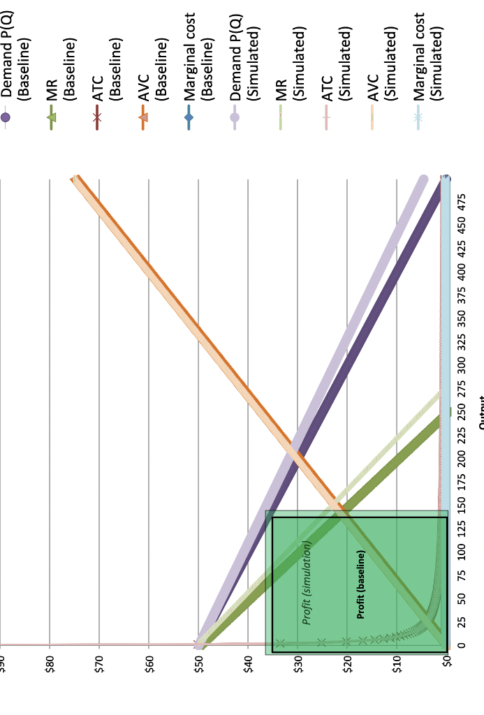
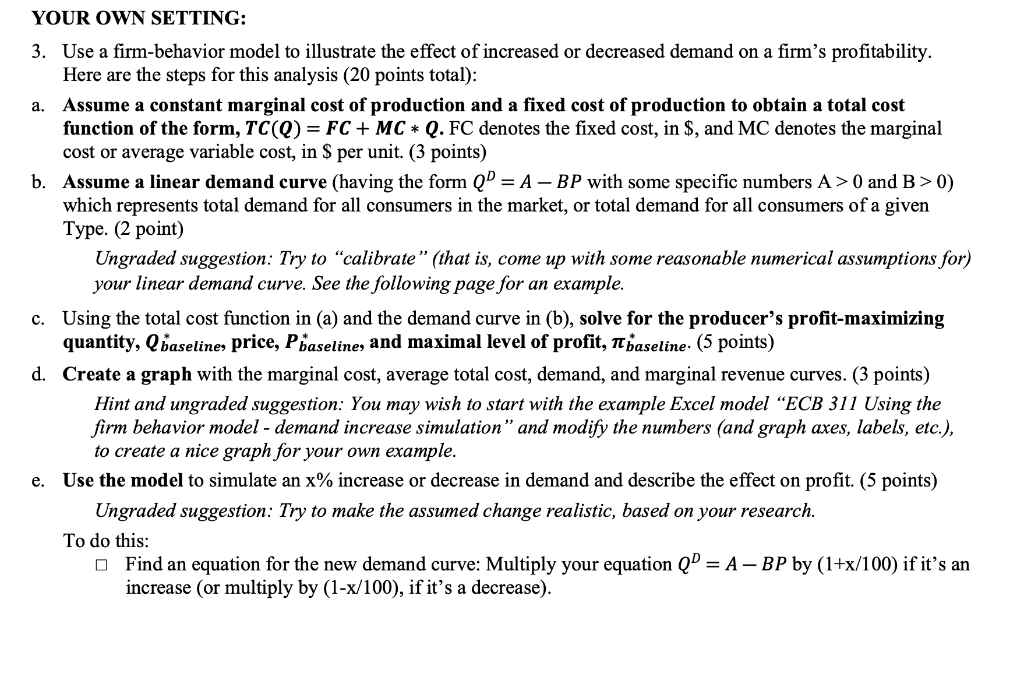
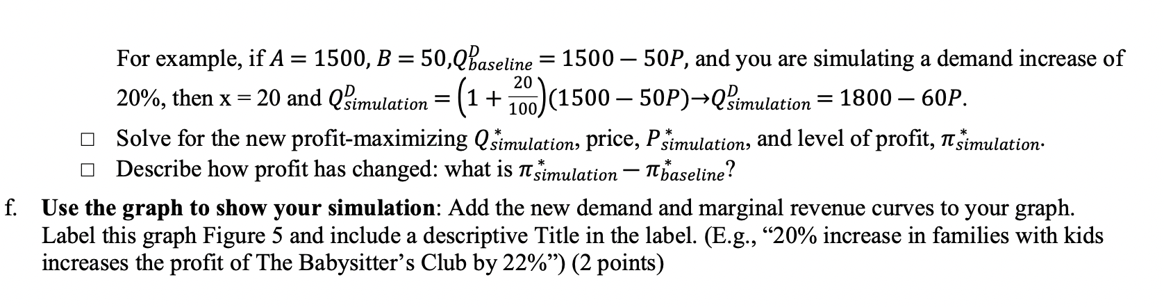
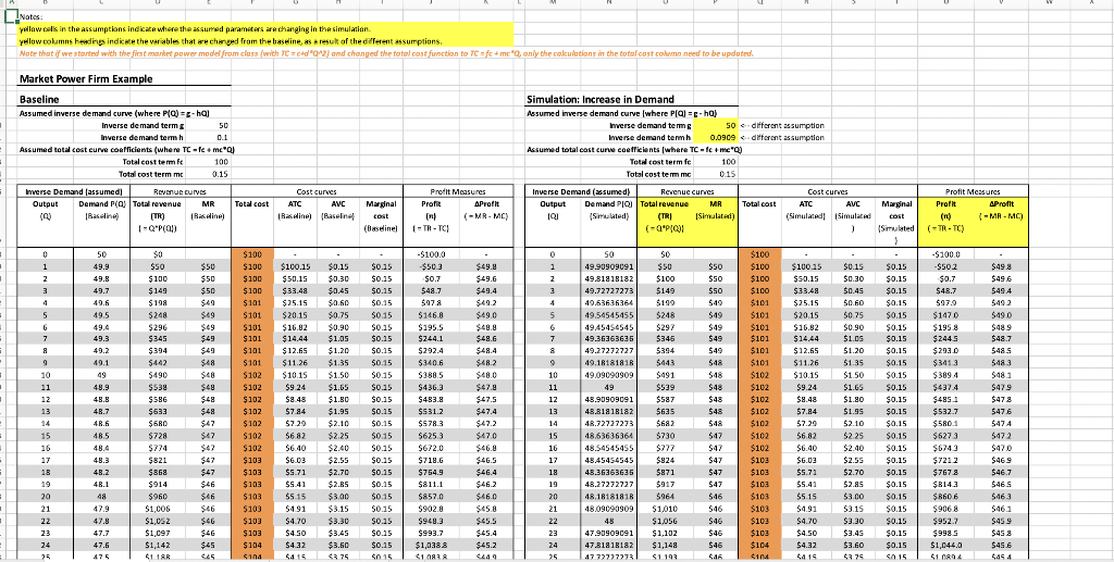
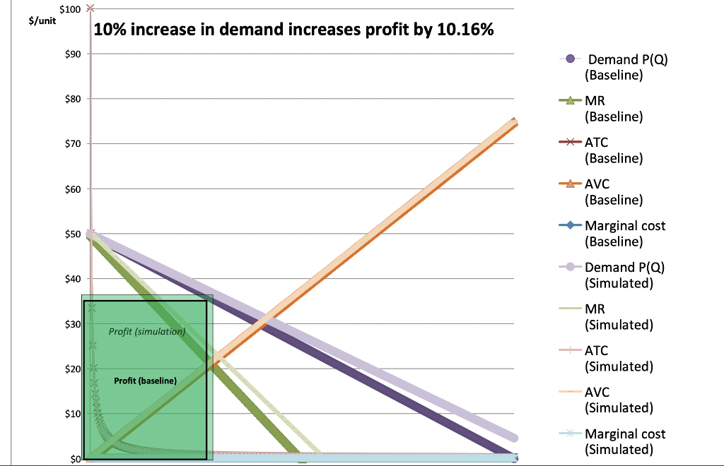
E $80 $70 $60 $50 $40 $30 Profit (simulation) $20 Profit (baseline) $10 $0 0 25 50 75 100 125 150 175 200 225 250 275 300 325 350 375 400 425 450 475 Output Demand P(Q) (Baseline) MR (Baseline) ATC (Baseline) -AVC (Baseline) Marginal cost (Baseline) Demand P(Q) (Simulated) (Simulated) (Simulated) AVC (Simulated) Marginal cost (Simulated) --MR ATC YOUR OWN SETTING: 3. Use a firm-behavior model to illustrate the effect of increased or decreased demand on a firm's profitability. Here are the steps for this analysis (20 points total): a. Assume a constant marginal cost of production and a fixed cost of production to obtain a total cost function of the form, TC(Q) = FC + MC * Q. FC denotes the fixed cost, in $, and MC denotes the marginal cost or average variable cost, in $ per unit. (3 points) b. Assume a linear demand curve (having the form QD = A - BP with some specific numbers A> 0 and B>0) which represents total demand for all consumers in the market, or total demand for all consumers of a given Type. (2 point) Ungraded suggestion: Try to "calibrate" (that is, come up with some reasonable numerical assumptions for) your linear demand curve. See the following page for an example. c. Using the total cost function in (a) and the demand curve in (b), solve for the producer's profit-maximizing quantity, Qbaseline, price, Phaseline, and maximal level of profit, baseline. (5 points) d. Create a graph with the marginal cost, average total cost, demand, and marginal revenue curves. (3 points) Hint and ungraded suggestion: You may wish to start with the example Excel model "ECB 311 Using the firm behavior model - demand increase simulation" and modify the numbers (and graph axes, labels, etc.), to create a nice graph for your own example. e. Use the model to simulate an x% increase or decrease in demand and describe the effect on profit. (5 points) Ungraded suggestion: Try to make the assumed change realistic, based on your research. To do this: Find an equation for the new demand curve: Multiply your equation QD = A - BP by (1+x/100) if it's an increase (or multiply by (1-x/100), if it's a decrease). For example, if A = 1500, B = 50,Qbaseline = 1500 - 50P, and you are simulating a demand increase of 1000) (15 (1500 50P)Qimulation = 1800 60P. 20 20%, then x 20 and Qsimulation = (1 + * Solve for the new profit-maximizing Qsimulation, price, Psimulation, and level of profit, simulation. Describe how profit has changed: what is simulation - baseline? L f. Use the graph to show your simulation: Add the new demand and marginal revenue curves to your graph. Label this graph Figure 5 and include a descriptive Title in the label. (E.g., 20% increase in families with kids increases the profit of The Babysitter's Club by 22%") (2 points) T | l t T 1 il il "I # 11 + :l ET || i il 1 T + Notes: yellow cells in the assumptions indicate where the assumed parameters are changing in the simulation. yellow columns headings indicate the variables that are changed from the baseline, as a result of the different assumptions. Note that if we started with the first market power model from class (with TC = c+d"Q^2) and changed the total cost function to TC = fc + mc*Q, only the calculations in the total cost column need to be updated. Market Power Firm Example Baseline Simulation: Increase in Demand Assumed inverse demand curve (where P(Q)-g-hQ) Inverse demand term 50 different assumption different assumption Inverse demand term h 0.1 Assumed total cost curve coefficients (where TC-fe+mc*Ql Total cost term fe 100 Total cost term mc Assumed inverse demand curve (where P[Q] =g-hQ) Inverse demand term g 50 Inverse demand term h 0.0909 Assumed total cost curve coefficients (where TC-fc+me"Q) Total cost term fe 100 Total cost term mc 0.15 Revenue curves Output Demand PIQ Total revenue MR Total cost [Q] (Simulated) (TR) Simulated) (=Q*P(Q) 0.15 Inverse Demand (assumed) Inverse Demand (assumed) Output Demand P(Q) Total revenue Total cost Cost curves ATC AVC Marginal (Baseline) (Baseline) cost (Baselinel Profit Measures Profit Aprofit [n) (-MR-MC) [Baseline) (TR) [-Q*P(Q) (-TR - IC 50 $100 -$100.0 0 $0 $50 1 49.9 $100 $100.15 $0.15 $0.15 $100 $50.15 $0.30 $0.15 $49.8 $49.6 2 49.8 -$50.3 -$0.7 $48.7 $100 3 49.7 $149 $49.4 4 49.6 $198 $100 $33.48 $0.45 $0.15 $25.15 $0.60 $0.15 $20.15 $0.75 $0.15 $97.8 $101 $101 $49.2 5 49.5 $248 $49.0 $146.8 $195.5 G 49.4 $296 $101 $16.82 $0.90 $0.15 $48.8 1 2 3 4 5 6 7 8 9 10 11 7 49.3 $345 $244.1 $48.6 $101 $14.44 $1.05 $0.15 $101 $12.65 $1.20 $0.15 49.2 $394 $292.4 $48.4 50 SO 49.90909091 $50 49.81818182 $100 49.72727273 $149 49.63636364 $199 49.54545455 $248 4945454545 $297 49.36363636 $345 49.27272727 $394 49.18181818 $443 49.09090909 $491 49 $539 48.90909091 $587 48.81818182 $635 48.72727273 $682 48.63636364 $730 48.54545455 $777 48.45454545 49.1 $442 $340.6 $48.2 $101 $102 49 $11.26 $1.35 $10.15 $102 $9.24 $490 $388.5 $48.0 $0.15 $1.50 $0.15 $1.65 $8.48 $1.80 48 9 $538 $436.3 $47.8 $0.15 $0.15 48.8 $586 $102 $483.8 $47.5 48.7 $633 $102 $7.84 $1.95 $0.15 $531.2 $47.4 12 13 14 48.6 $680 $102 $578.3 $47.2 $7.29 $2.10 $0.15 $6.82 $2.25 $0.15 48.5 $728 $102 $625.3 $47.0 15 48.4 $774 $672.0 $46.8 $102 $6.40 $103 $2.40 $0.15 $6.03 $2.55 $0.15 48.3 $821 $718.6 $46.5 $824 48.2 $868 $103 $5.71 $2.70 $0.15 $754.9 $46.4 48.36363636 $871 48.1 $914 $103 $5.41 $0.15 $811.1 $46.2 $917 $2.85 $3.00 $0.15 48.27272727 48.18181818 48 $960 $103 $5.15 $857.0 $46.0 $964 47.9 $1,006 $103 $4.91 $3.15 $0.15 $902.8 $45.8 48.09090909 $1,010 48 47.8 $1,052 $4.70 $3.30 $0.15 $948.3 $45.5 $103 $103 $4.50 $3.45 $0.15 47.7 $1,097 $993.7 $45.4 $1,056 47.90909091 $1,102 47.81818182 $1,148 $1.193 47.6 $1,142 $45.2 $104 $4.32 $3.60 $0.15 $1,0388 $1,083.8 475 $1.18R $104 $4.15 $3.75 $0.15 $449 47.72727273 8 9 10 11 12 13 14 15 16 17 18 19 20 21 22 23 24 25 Revenue curves MR [Baseline) $50 $50 $50 $49 $49 $49 $49 $49 $48 S48 $48 $48 $48 $47 $47 $47 $47 $47 $46 $46 $46 $46 $46 $45 45 *=*=*=*=*: 75 Cost curves ATC AVC Marginal (Simulated) (Simulated 1 (Simulated 1 $0.15 $0.30 $0.15 $0.45 $0.15 50.60 $0.15 $0.75 $0.15 $0.90 $0.15 $1.05 $0.15 $100 $50 $100 $100.15 $0.15 $50 $100 $50.15 $50 $100 $33.48 $49 $101 $25.15 $49 $101 $20.15 $49 $101 $16.82 $49 $101 $14.44 $49 $101 $12.65 $48 $101 $11.26 $48 $102 $10.15 $48 $9.24 $48 $8.48 $48 $48 $47 $1.20 $0.15 $1.35 $0.15 $1.50 $0.15 $1.65 $0.15 $102 $102 $1.80 $0.15 $102 $7.84 $1.95 $0.15 $102 $7.29 $2.10 $0.15 $102 56.82 $2.25 $0.15 $47 $102 $2.40 $0.15 $47 $103 $47 $103 $6.40 $6.03 $5.71 $5.41 $5.15 $2.55 $0.15 $2.70 $0.15 $2.85 $0.15 547 $103 $46 $103 $3.00 $0.15 $46 $103 $4.91 $3.15 $0.15 $46 $103 $3.30 $0.15 $4.70 $4.50 $103 $46 $46 $46 $3.43 $0.15 $3.60 $0.15 $104 $4.32 $4.15 $104 $3.75 $0.15 Profit Measures Profit Aprofit (n) (-MR-MC) (-TR-TC) -$100.0 -$50.2 $49.8 $49.6 $0.7 $49.4 $48.7 $97.9 $49.2 $147.0 $49.0 $48.9 $195.8 $244.5 $293.0 $48.7 $48.5 $341.3 $48.3 $389.4 $48.1 $437.4 $47.9 $485.1 $47.8 $532.7 $47.6 $580.1 $47.4 $627.3 $47.2 $674.3 $47.0 $7212 $46.9 $767.8 $46.7 $814.3 $46.5 $860.6 $46.3 $906.8 $46.1 $952.7 $45.9 $45.8 $998.5 $1,044.0 $1.089.4 $45.6 $45 4 $100 $/unit 10% increase in demand increases profit by 10.16% $90 $80 $70 $60 $50 $40 $30 $20 $10 $0 Profit (simulation) Profit (baseline) Demand P(Q) (Baseline) MR (Baseline) (Baseline) AVC (Baseline) Marginal cost (Baseline) Demand P(Q) (Simulated) MR (Simulated) ATC (Simulated) AVC (Simulated) Marginal cost (Simulated) ATC E $80 $70 $60 $50 $40 $30 Profit (simulation) $20 Profit (baseline) $10 $0 0 25 50 75 100 125 150 175 200 225 250 275 300 325 350 375 400 425 450 475 Output Demand P(Q) (Baseline) MR (Baseline) ATC (Baseline) -AVC (Baseline) Marginal cost (Baseline) Demand P(Q) (Simulated) (Simulated) (Simulated) AVC (Simulated) Marginal cost (Simulated) --MR ATC YOUR OWN SETTING: 3. Use a firm-behavior model to illustrate the effect of increased or decreased demand on a firm's profitability. Here are the steps for this analysis (20 points total): a. Assume a constant marginal cost of production and a fixed cost of production to obtain a total cost function of the form, TC(Q) = FC + MC * Q. FC denotes the fixed cost, in $, and MC denotes the marginal cost or average variable cost, in $ per unit. (3 points) b. Assume a linear demand curve (having the form QD = A - BP with some specific numbers A> 0 and B>0) which represents total demand for all consumers in the market, or total demand for all consumers of a given Type. (2 point) Ungraded suggestion: Try to "calibrate" (that is, come up with some reasonable numerical assumptions for) your linear demand curve. See the following page for an example. c. Using the total cost function in (a) and the demand curve in (b), solve for the producer's profit-maximizing quantity, Qbaseline, price, Phaseline, and maximal level of profit, baseline. (5 points) d. Create a graph with the marginal cost, average total cost, demand, and marginal revenue curves. (3 points) Hint and ungraded suggestion: You may wish to start with the example Excel model "ECB 311 Using the firm behavior model - demand increase simulation" and modify the numbers (and graph axes, labels, etc.), to create a nice graph for your own example. e. Use the model to simulate an x% increase or decrease in demand and describe the effect on profit. (5 points) Ungraded suggestion: Try to make the assumed change realistic, based on your research. To do this: Find an equation for the new demand curve: Multiply your equation QD = A - BP by (1+x/100) if it's an increase (or multiply by (1-x/100), if it's a decrease). For example, if A = 1500, B = 50,Qbaseline = 1500 - 50P, and you are simulating a demand increase of 1000) (15 (1500 50P)Qimulation = 1800 60P. 20 20%, then x 20 and Qsimulation = (1 + * Solve for the new profit-maximizing Qsimulation, price, Psimulation, and level of profit, simulation. Describe how profit has changed: what is simulation - baseline? L f. Use the graph to show your simulation: Add the new demand and marginal revenue curves to your graph. Label this graph Figure 5 and include a descriptive Title in the label. (E.g., 20% increase in families with kids increases the profit of The Babysitter's Club by 22%") (2 points) T | l t T 1 il il "I # 11 + :l ET || i il 1 T + Notes: yellow cells in the assumptions indicate where the assumed parameters are changing in the simulation. yellow columns headings indicate the variables that are changed from the baseline, as a result of the different assumptions. Note that if we started with the first market power model from class (with TC = c+d"Q^2) and changed the total cost function to TC = fc + mc*Q, only the calculations in the total cost column need to be updated. Market Power Firm Example Baseline Simulation: Increase in Demand Assumed inverse demand curve (where P(Q)-g-hQ) Inverse demand term 50 different assumption different assumption Inverse demand term h 0.1 Assumed total cost curve coefficients (where TC-fe+mc*Ql Total cost term fe 100 Total cost term mc Assumed inverse demand curve (where P[Q] =g-hQ) Inverse demand term g 50 Inverse demand term h 0.0909 Assumed total cost curve coefficients (where TC-fc+me"Q) Total cost term fe 100 Total cost term mc 0.15 Revenue curves Output Demand PIQ Total revenue MR Total cost [Q] (Simulated) (TR) Simulated) (=Q*P(Q) 0.15 Inverse Demand (assumed) Inverse Demand (assumed) Output Demand P(Q) Total revenue Total cost Cost curves ATC AVC Marginal (Baseline) (Baseline) cost (Baselinel Profit Measures Profit Aprofit [n) (-MR-MC) [Baseline) (TR) [-Q*P(Q) (-TR - IC 50 $100 -$100.0 0 $0 $50 1 49.9 $100 $100.15 $0.15 $0.15 $100 $50.15 $0.30 $0.15 $49.8 $49.6 2 49.8 -$50.3 -$0.7 $48.7 $100 3 49.7 $149 $49.4 4 49.6 $198 $100 $33.48 $0.45 $0.15 $25.15 $0.60 $0.15 $20.15 $0.75 $0.15 $97.8 $101 $101 $49.2 5 49.5 $248 $49.0 $146.8 $195.5 G 49.4 $296 $101 $16.82 $0.90 $0.15 $48.8 1 2 3 4 5 6 7 8 9 10 11 7 49.3 $345 $244.1 $48.6 $101 $14.44 $1.05 $0.15 $101 $12.65 $1.20 $0.15 49.2 $394 $292.4 $48.4 50 SO 49.90909091 $50 49.81818182 $100 49.72727273 $149 49.63636364 $199 49.54545455 $248 4945454545 $297 49.36363636 $345 49.27272727 $394 49.18181818 $443 49.09090909 $491 49 $539 48.90909091 $587 48.81818182 $635 48.72727273 $682 48.63636364 $730 48.54545455 $777 48.45454545 49.1 $442 $340.6 $48.2 $101 $102 49 $11.26 $1.35 $10.15 $102 $9.24 $490 $388.5 $48.0 $0.15 $1.50 $0.15 $1.65 $8.48 $1.80 48 9 $538 $436.3 $47.8 $0.15 $0.15 48.8 $586 $102 $483.8 $47.5 48.7 $633 $102 $7.84 $1.95 $0.15 $531.2 $47.4 12 13 14 48.6 $680 $102 $578.3 $47.2 $7.29 $2.10 $0.15 $6.82 $2.25 $0.15 48.5 $728 $102 $625.3 $47.0 15 48.4 $774 $672.0 $46.8 $102 $6.40 $103 $2.40 $0.15 $6.03 $2.55 $0.15 48.3 $821 $718.6 $46.5 $824 48.2 $868 $103 $5.71 $2.70 $0.15 $754.9 $46.4 48.36363636 $871 48.1 $914 $103 $5.41 $0.15 $811.1 $46.2 $917 $2.85 $3.00 $0.15 48.27272727 48.18181818 48 $960 $103 $5.15 $857.0 $46.0 $964 47.9 $1,006 $103 $4.91 $3.15 $0.15 $902.8 $45.8 48.09090909 $1,010 48 47.8 $1,052 $4.70 $3.30 $0.15 $948.3 $45.5 $103 $103 $4.50 $3.45 $0.15 47.7 $1,097 $993.7 $45.4 $1,056 47.90909091 $1,102 47.81818182 $1,148 $1.193 47.6 $1,142 $45.2 $104 $4.32 $3.60 $0.15 $1,0388 $1,083.8 475 $1.18R $104 $4.15 $3.75 $0.15 $449 47.72727273 8 9 10 11 12 13 14 15 16 17 18 19 20 21 22 23 24 25 Revenue curves MR [Baseline) $50 $50 $50 $49 $49 $49 $49 $49 $48 S48 $48 $48 $48 $47 $47 $47 $47 $47 $46 $46 $46 $46 $46 $45 45 *=*=*=*=*: 75 Cost curves ATC AVC Marginal (Simulated) (Simulated 1 (Simulated 1 $0.15 $0.30 $0.15 $0.45 $0.15 50.60 $0.15 $0.75 $0.15 $0.90 $0.15 $1.05 $0.15 $100 $50 $100 $100.15 $0.15 $50 $100 $50.15 $50 $100 $33.48 $49 $101 $25.15 $49 $101 $20.15 $49 $101 $16.82 $49 $101 $14.44 $49 $101 $12.65 $48 $101 $11.26 $48 $102 $10.15 $48 $9.24 $48 $8.48 $48 $48 $47 $1.20 $0.15 $1.35 $0.15 $1.50 $0.15 $1.65 $0.15 $102 $102 $1.80 $0.15 $102 $7.84 $1.95 $0.15 $102 $7.29 $2.10 $0.15 $102 56.82 $2.25 $0.15 $47 $102 $2.40 $0.15 $47 $103 $47 $103 $6.40 $6.03 $5.71 $5.41 $5.15 $2.55 $0.15 $2.70 $0.15 $2.85 $0.15 547 $103 $46 $103 $3.00 $0.15 $46 $103 $4.91 $3.15 $0.15 $46 $103 $3.30 $0.15 $4.70 $4.50 $103 $46 $46 $46 $3.43 $0.15 $3.60 $0.15 $104 $4.32 $4.15 $104 $3.75 $0.15 Profit Measures Profit Aprofit (n) (-MR-MC) (-TR-TC) -$100.0 -$50.2 $49.8 $49.6 $0.7 $49.4 $48.7 $97.9 $49.2 $147.0 $49.0 $48.9 $195.8 $244.5 $293.0 $48.7 $48.5 $341.3 $48.3 $389.4 $48.1 $437.4 $47.9 $485.1 $47.8 $532.7 $47.6 $580.1 $47.4 $627.3 $47.2 $674.3 $47.0 $7212 $46.9 $767.8 $46.7 $814.3 $46.5 $860.6 $46.3 $906.8 $46.1 $952.7 $45.9 $45.8 $998.5 $1,044.0 $1.089.4 $45.6 $45 4 $100 $/unit 10% increase in demand increases profit by 10.16% $90 $80 $70 $60 $50 $40 $30 $20 $10 $0 Profit (simulation) Profit (baseline) Demand P(Q) (Baseline) MR (Baseline) (Baseline) AVC (Baseline) Marginal cost (Baseline) Demand P(Q) (Simulated) MR (Simulated) ATC (Simulated) AVC (Simulated) Marginal cost (Simulated) ATC