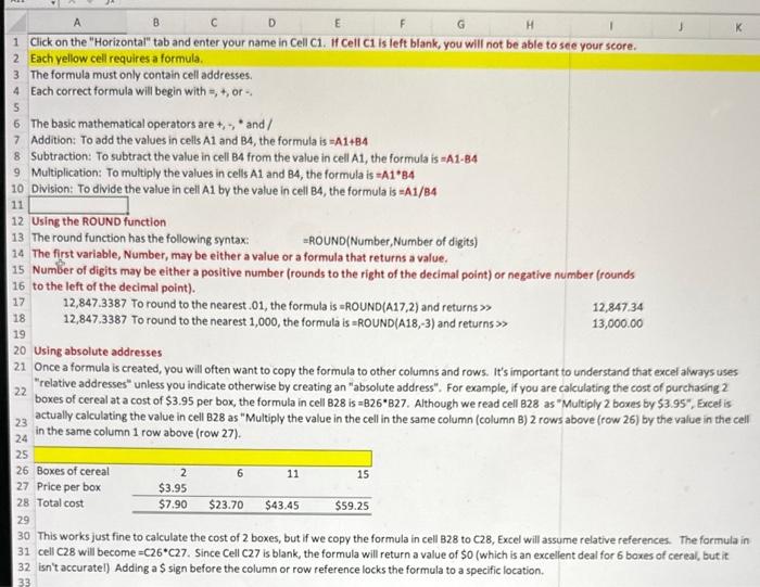
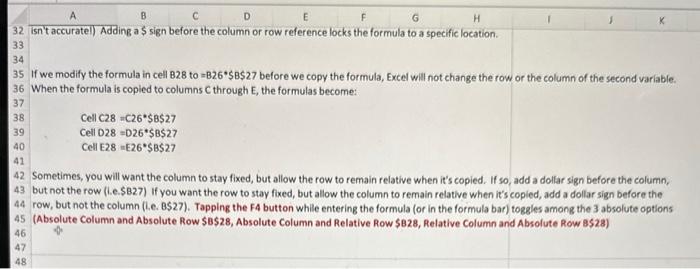
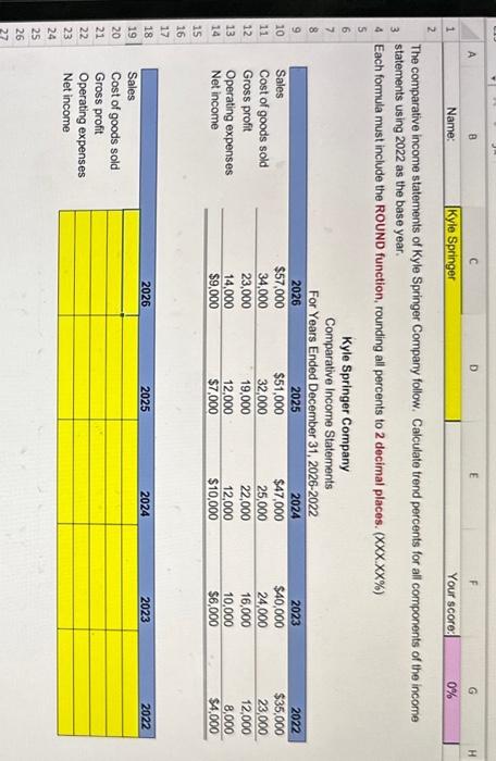Each yellow cell requires a formula. The formula must only contain cell addresses. Each correct formula will begin with =,+, or , The basic mathematical operators are +,,+ and / Addition: To add the values in cells A1 and BA, the formula is =A1+BA Subtraction: To subtract the value in cell B4 from the value in cell A1, the formula is =A1-B4 Multiplication: To multiply the values in cells A1 and B4, the formula is =A1B4 Division: To divide the value in cell A1 by the value in cell BA, the formula is =A1/B4 Using the ROUND function The round function has the following syntax: =ROUND(Number, Number of digits) The first variable, Number, may be either a value or a formula that returns a value. Number of digits may be either a positive number (rounds to the right of the decimal point) or negative number (rounds to the left of the decimal point). 12,847.3387Toroundtothenearest.01,theformulaisaROUND(A17,2)andreturns>12,847.3387Toroundtothenearest1,000,theformulais=ROUND(A18,3)andreturns>12,847.3413,000.00 Using absolute addresses Once a formula is created, you will often want to copy the formula to other columns and rows. It's important to understand that excel always uses "relative addresses" unless you indicate otherwise by creating an "absolute address". For example, if you are calculating the cost of purchasing 2 boxes of cereal at a cost of $3.95 per box, the formula in cell 828 is =826827. Although we read cell 828 as "Multiply 2 boxes by $3.95, Excel is actually calculating the value in cell 828 as "Multiply the value in the cell in the same column (column B ) 2 rows above (row 26 ) by the value in the cell in the same column 1 row above (row 27). This works just fine to calculate the cost of 2 boxes, but if we copy the formula in cell 328 to C28, Excel will assume relative references. The formula in cell C28 will become =C26C27. Since Cell C27 is blank, the formula will return a value of $0 (which is an excellent deal for 6 boxes of cereal, but it isn't accuratel) Adding a $ sign before the column or row reference locks the formula to a specific location. Isn't accuratel) Adding a $ sign before the column of row reference locks the formula to a specific location. If we modify the formula in cell B28 to =B26$B$27 before we copy the formula, Excel will not change the row or the column of the second variable. When the formula is copied to columns C through E, the formulas become: CellC28=C26$8$27CellD28=D26$B27CellE28=E26$B$27 Sometimes, you will want the column to stay fixed, but allow the row to remain relative when it's copied. If so, add a dolfar sign before the column, but not the row (L.e.\$827) If you want the row to stay fixed, but allow the column to remain relative when it's copied, add a dollar sign before the row, but not the column (L.e. BS27). Tapping the F4 button while entering the formula (or in the formula bar) toggles among the 3 absolute options (Absolute Column and Absolute Row \$8\$28, Absolute Column and Relative Row \$828, Relative Column and Absolute Row 8 \$28) The comparative income statements of Kyle Springer Company follow. Calculate trend percents for all components of the income statements using 2022 as the base year. Each formula must include the ROUND function, rounding all percents to 2 decimal places. ( XXXXXX% )