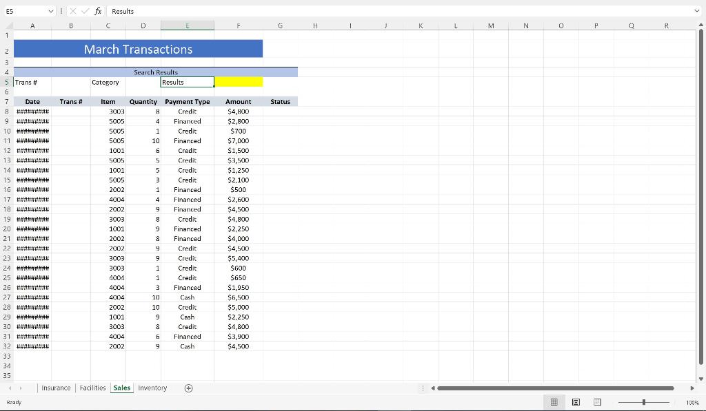
Ensure the Sales worksheet is active. Enter a function in cell B8 to create a custom transaction number. The transaction number should be comprised of the item number listed in cell C8 combined with the quantity in cell D8 and the first initial of the payment type in cell E8. Use Auto Fill to copy the function down, completing the data in column B. Hint: The function is =C8&D8&LEFT(E8,1). -Sales Worksheet active -Function created in B8 -Function returns -item number listed in cell C8 -combined with the quantity in cell D8 and -the first initial of the payment type in cell E8. -Auto Fill used to copy the above function down to complete in column B

Enter a nested function in cell G8 that displays the word Flag if the Payment Type is Credit and the Amount is greater than or equal to $4000. Otherwise, the function will display a blank cell. Use Auto Fill to copy the function down, completing the data in column G. Hint: The function is =IF (AND (logical 1, logical 2....), ) For example: IF (AND (E8="Credit", logic 2),"Flag","") -Nested function in cell G8 has correct criteria -Nested function in cell G8 has correct cell references -Nested function in cell G8, displays word "Flag" if -Payment Type is Credit and - Amount is greater than or equal to $4000 -Nested function in cell G8, displays a blank cell for other conditions -Auto Fill used to copy the above function down to complete in column G

Create a data validation list in cell D5 that displays Quantity, Payment Type, and Amount. Hint: On the Data tab, in the Data Tools group, click Data Validation, Allow, List -Data list created in cell D5 -List has Quantity, Payment Type, and Amount

Type the Trans# 30038C in cell B5, and select Quantity from the validation list in cell D5. Hint: -Trans# 30038C in cell B5 -Validation List Quantity displayed in cell D5

Enter a nested lookup function in cell F5 that evaluates the Trans # in cell B5 as well as the Category in cell D5, and returns the results based on the data in the range A8:F32. Hint: Use function INDEX() and MATCH(). -Nested lookup function in cell F5 -Evaluates Trans # in cell B5, Category in cell D5 -Returns results based on date in range A8:F32

Create a PivotTable based on the range A7:G32. Place the PivotTable in cell I17 on the current worksheet. Place Payment Type in the Rows box and Amount in the Values box. Format the Amount with Accounting Number Format. Hint: On the Insert tab, in the Tables group, select PivotTable. -Range A7:G32 used to create PivotTable -PivotTable placed in cell I17 in current worksheet -Payment Type in the Rows box area -Amount in the Values box area -Amount formatted with Accounting Format

Insert a PivotChart using the Pie chart type based on the data. Place the upper-left corner of the chart inside cell I22. Format the Legend of the chart to appear at the bottom of the chart area. Format the Data Labels to appear on the Outside end of the chart. Hint: On the Analyze tab, in the Tools group, click PivotChart. -Create PivotChart Pie Chart based on above data -Upper-left corner of the PivotChart Pie Chart placed in cell I22 -Legend of PivotChart formatted to appear at the bottom of Chart area -Data Labels to appear on the Outside end of the chart

Insert a Slicer based on Date. Place the upper-left corner of the Slicer inside cell L8. Hint: On the Insert tab, in the Filters group, and click Slicer. -Slicer based on Date from PivotTable -Upper-left corner of the Slicer in cell L8 -Slicer has right values

Having trouble with the instructions for this practice sales worksheet, help?

Link to Excel File is in the comments :)

https://1drv.ms/x/s!AtHepBTmkrg2jyEAv9Zwomniv9xB?e=FdmYzB

E5 fx Results A D D G H 1 M N 0 P 0 R 1 2 March Transactions Status Financed 3 Search Results 5 Trans # Category Results 6 7 Date Trans # Item Quantity Payment Type 8 # 3003 B Credit 9 #14 5005 4 Financed 10 #### 5005 1 Credit 11 5005 10 Financed 12 11 1001 6 Credit 13 WMA 5005 5 Credit 14 ##### 1001 5 Credit 15 ######## 5005 3 Credit 16 ######## 2002 1 Financed 17 ##### 4004 4 18 WAHHAAH 2002 9 Financed 19 ######## 3003 8 Credit 20 ##### 1001 9 Financed 21 ##### 2002 8 Financed 22 2002 9 Credit 23 HAWWAA 3003 9 Credit 24 ######### 3003 1 Credit 25 ######### 4004 1 Credit 26 ### 4004 3 Financed 27 MAH 4004 10 Cash 28 WW#### 2002 10 Credit 29 ######### 1001 9 Cash 30 ##### 3003 8 Credit 31 4004 6 Financed 32 AM 2002 9 Cash 33 34 35 Insurance Facilities Sales Inventory Raacy Amount $4,400 $2,800 $700 $7,000 $1,500 $3,500 $1,250 $2,100 $500 $2,600 $4,500 $4,800 $2,250 $4,000 $4,500 $5,400 $600 $650 $1,950 $6,500 $5,000 $2,250 $4,800 $3,900 $4,500 16 1 100%