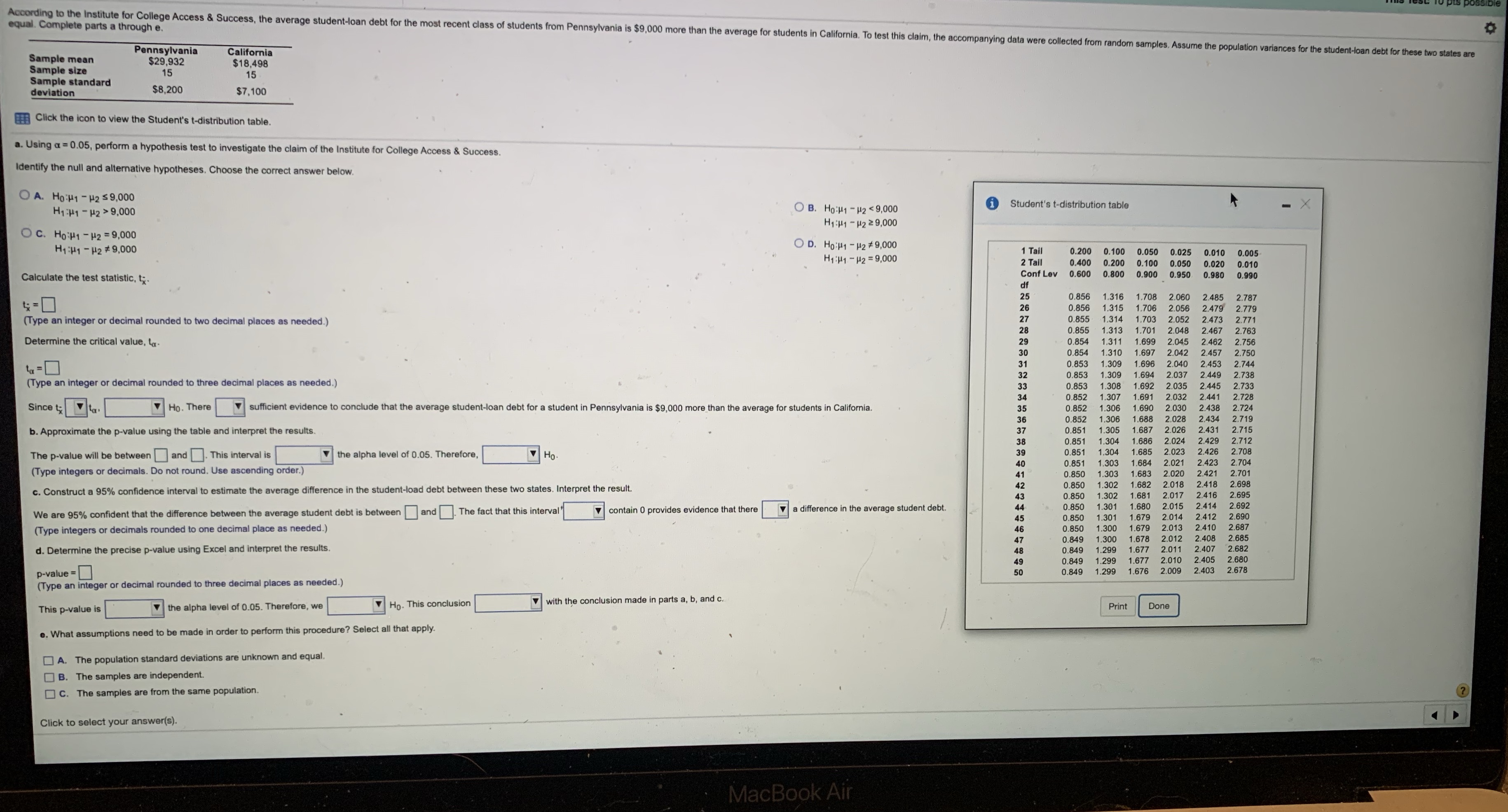
equal. Complete parts a through e. According to the Institute for College Access & Success, the average student-loan debt for the most recent class of students from Pennsylvania is $9,000 more than the average for students in California. To test this claim, the accompanying data were collected from random samples. Assume the population variances for the student-loan debt for these two states are Pennsylvania California Sample mean $29,932 $18,498 Sample size 15 15 Sample standard deviation $8,200 $7,100 Click the icon to view the Student's t-distribution table. a. Using a = 0.05, perform a hypothesis test to investigate the claim of the Institute for College Access & Success. Identify the null and alternative hypotheses. Choose the correct answer below. O A. Ho:H1 - H2 $ 9,000 O B. Ho:H1 - H2 9,000 Student's t-distribution table H1:141 - H2 2 9,000 O C. Ho:H1 - H2 = 9,000 H1:141 - H2 #9,000 O D. Ho:H1 - H2 #9,000 1 Tail 0.200 0.100 0.050 0.025 0.010 0.005 H1:141 - H2 =9,000 2 Tail 0.400 0.200 0.100 0.050 0.020 0.010 Calculate the test statistic, t. Conf Lev 0.600 0.800 0.900 0.950 0.980 0.990 df 25 0.856 1,316 1.708 2.060 2.485 2.787 26 0.856 1.315 1.706 2.056 2.479 2.779 (Type an integer or decimal rounded to two decimal places as needed.) 27 0.855 1.314 1.703 2.052 2.473 2.771 28 0.855 1.313 3 1.701 2.048 2.467 2.763 Determine the critical value, tax 29 0.854 1.311 1.699 2.045 2.462 2.756 30 0.854 1.310 1.697 2.042 2.457 2.750 ta = 0 31 0.853 1.309 1.696 2.040 2.453 2.744 32 0.853 1.309 1.694 2.037 2.449 2.738 (Type an integer or decimal rounded to three decimal places as needed.) 33 0.853 1.308 1.692 2.035 2.445 2.733 34 0.85 1.307 2.032 2.441 2.728 Since ta ta. Ho. There sufficient evidence to conclude that the average student-loan debt for a student in Pennsylvania is $9,000 more than the average for students in California. 35 0.852 1.306 1.690 2.030 2.438 2.724 36 0.852 1.306 2.028 2434 2.719 b. Approximate the p-value using the table and interpret the results. 37 0.851 1.305 2.026 2.431 2.715 38 0.851 1.304 1.686 2.024 2.429 2.712 The p-value will be between ] and . This interval is the alpha level of 0.05. Therefore, V Ho 39 0.851 1.304 2.023 2.426 2.708 40 0.851 1.303 1.684 2.021 2.423 2.704 (Type integers or decimals. Do not round. Use ascending order.) 41 0.850 1.303 1.683 2.020 2.421 2.701 42 0.850 1.302 1.682 2.018 2.418 2.698 c. Construct a 95% confidence interval to estimate the average difference in the student-load debt between these two states. Interpret the result. 43 0.850 1.302 1.681 2.017 2.416 2.695 We are 95% confident that the difference between the average student debt is between ] and . The fact that this interval' contain 0 provides evidence that there |a difference in the average student debt. 44 0.850 1.301 1.680 2.015 2.414 2.692 45 0.850 1.301 1.679 2.014 2.412 2.690 (Type integers or decimals rounded to one decimal place as needed.) 0.850 1.300 1.679 2.013 2.410 2.687 0.849 1.300 1.678 2.012 2.408 2.685 d. Determine the precise p-value using Excel and interpret the results. 48 0.849 1.299 1.677 2.011 2.407 2.682 49 0.849 1.299 1.677 2.010 2.405 2. 2.680 p-value = 50 0.849 1.299 1.676 2.009 2.403 2.678 (Type an integer or decimal rounded to three decimal places as needed.) the alpha level of 0.05. Therefore, we Ho- This conclusion with the conclusion made in parts a, b, and c. This p-value is Print Done e. What assumptions need to be made in order to perform this procedure? Select all that apply. A. The population standard deviations are unknown and equal. B. The samples are independent. C. The samples are from the same population. Click to select your answer(s). MacBook Air


