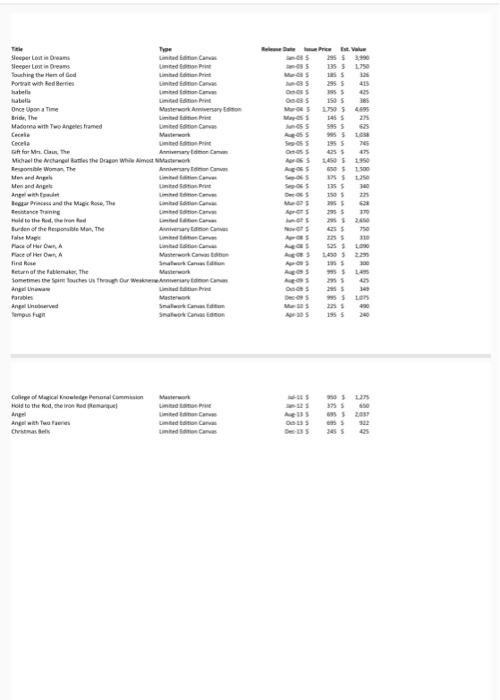
EX16 XL CHO5 GRADER CAP HW Fine Art 1.9 Project Description: Project Description> Instructions: For the purpose of grading the project you are required to perform the following tasks: Start Excel. Open the downloaded Excel file named exploring eo5 grader_hl startxisx. Save the workbook as exploring e05 grader hl LastFirst, replacing LastFirst with your own name. On the Subtotals worksheet, sort the data by Type and further sort it by Title, both in alphabetical order Use the Subtotals feature to insert subtotal rows by Type to identify the highest Issue Price and Est. Value. Collapse the data by displaying only the subtotals and grand total rows. Set a print area for the range B1:E45 Use the Art worksheet to create a blank PivotTable on a new worksheet named Sold Out. Name the PivotTable Average Price by Type. Use the Type and Issue Price fields, enabling Excel to determine where the fields go in the PivotTable. Add the Est. Value field to the Values area. s to determine the average I ce and average Value by type. Change the custom name to Average Issue Price and Average Est. Value, respectively 8 Format the two Values fields with Currency number type with zero decimal places a ca difference between the two values, Est. Value and Issue Price. Move the calculated field up so that it displays in Column C (Hint: Click on the drop-down option of the field name in the PivotTable Fields pane, and then click Move Up). For the calculated field, use the custom name Percentage Change in Value. Apply Percentage number format with two decimal places Select the range B3:D3 and apply these formats: wrap text and Align Right horizontal alignment. Set the height of Row 3 to 60 and set the width of Columns B through D to 10. (Columns B:D). Type Type of Art in cell A3 and Average of A Art in cell All Updated: 11/09/2017 Step Move the Sold Out field from the field list to the Filters area. Set a filter to display only sold-out art (indicated by Yes). 12 Apply Light Blue, Pivot Style Light 23 and display banded columns. Note, depending upon Office version used, style name may be Pivot Style Light 23. apply the Light Blue, Slicer Style Dark 1. Move the slider below the PivotTable. 13 cer 14 Note, depending upon the Office version used, the style name may be Slicer Style Dark 1 Insert a timeline for the Release Date field, change the time period to YEARS, 15 change the timeline width to 4 inches, and move the timeline below the slicer Note, Mac users continue to the next step. e a c the to a new sheet named PivotChart. Hide the field buttons in the PivotChart 16 Note, Mac users, select the range A3:D10 and insert a clustered bar chart. Ensure that the legend displays the field names from row 3, and then move the chart to a new sheet named PivotChart. 17 Add a chart title and type Values for Sold-Out Art. Apply chart Style 12. 18 Apply 11 pt font size to the value axis and the legend. Create a footer on all worksheets (except Art) with your name in the left section, 19 the sheet name code in the center section, and the file name code in the right Ensure that the worksheets are correctly named and placed in the following order in the workbook: Subtotals, PivotChart, Sold Out, Art. Save the workbook. Close the workbook and then exit Excel. Submit the workbook as directed. 20 Total Points Updated: 11/092017 Madorea with Two ingeles framed Midhael the Archangel Bames the Dragon Whie Amt NMasterwok egar Princess and the Magic Ros, The Smalwork Caas 051352 haue Price t Value Masterwork Annivenary Edition Madonna with Twe ingeles framed Mchaelthe Archangel Bottles the Dragen While imost NMasterwok Beggar Princess and the Magc Rose, The urden of the Responsible Man, The Sometimes the Spit Touches Us Theough Our College ofMagical wedge Personal Commssien old to the Rod, the Inon Rod (Remarque $ 950 1,275 s 375 % 650 Masterwok 695 2,03 Oct-13 Limited Avalabl 5 695 922 $ 245 425 EX16 XL CHO5 GRADER CAP HW Fine Art 1.9 Project Description: Project Description> Instructions: For the purpose of grading the project you are required to perform the following tasks: Start Excel. Open the downloaded Excel file named exploring eo5 grader_hl startxisx. Save the workbook as exploring e05 grader hl LastFirst, replacing LastFirst with your own name. On the Subtotals worksheet, sort the data by Type and further sort it by Title, both in alphabetical order Use the Subtotals feature to insert subtotal rows by Type to identify the highest Issue Price and Est. Value. Collapse the data by displaying only the subtotals and grand total rows. Set a print area for the range B1:E45 Use the Art worksheet to create a blank PivotTable on a new worksheet named Sold Out. Name the PivotTable Average Price by Type. Use the Type and Issue Price fields, enabling Excel to determine where the fields go in the PivotTable. Add the Est. Value field to the Values area. s to determine the average I ce and average Value by type. Change the custom name to Average Issue Price and Average Est. Value, respectively 8 Format the two Values fields with Currency number type with zero decimal places a ca difference between the two values, Est. Value and Issue Price. Move the calculated field up so that it displays in Column C (Hint: Click on the drop-down option of the field name in the PivotTable Fields pane, and then click Move Up). For the calculated field, use the custom name Percentage Change in Value. Apply Percentage number format with two decimal places Select the range B3:D3 and apply these formats: wrap text and Align Right horizontal alignment. Set the height of Row 3 to 60 and set the width of Columns B through D to 10. (Columns B:D). Type Type of Art in cell A3 and Average of A Art in cell All Updated: 11/09/2017 Step Move the Sold Out field from the field list to the Filters area. Set a filter to display only sold-out art (indicated by Yes). 12 Apply Light Blue, Pivot Style Light 23 and display banded columns. Note, depending upon Office version used, style name may be Pivot Style Light 23. apply the Light Blue, Slicer Style Dark 1. Move the slider below the PivotTable. 13 cer 14 Note, depending upon the Office version used, the style name may be Slicer Style Dark 1 Insert a timeline for the Release Date field, change the time period to YEARS, 15 change the timeline width to 4 inches, and move the timeline below the slicer Note, Mac users continue to the next step. e a c the to a new sheet named PivotChart. Hide the field buttons in the PivotChart 16 Note, Mac users, select the range A3:D10 and insert a clustered bar chart. Ensure that the legend displays the field names from row 3, and then move the chart to a new sheet named PivotChart. 17 Add a chart title and type Values for Sold-Out Art. Apply chart Style 12. 18 Apply 11 pt font size to the value axis and the legend. Create a footer on all worksheets (except Art) with your name in the left section, 19 the sheet name code in the center section, and the file name code in the right Ensure that the worksheets are correctly named and placed in the following order in the workbook: Subtotals, PivotChart, Sold Out, Art. Save the workbook. Close the workbook and then exit Excel. Submit the workbook as directed. 20 Total Points Updated: 11/092017 Madorea with Two ingeles framed Midhael the Archangel Bames the Dragon Whie Amt NMasterwok egar Princess and the Magic Ros, The Smalwork Caas 051352 haue Price t Value Masterwork Annivenary Edition Madonna with Twe ingeles framed Mchaelthe Archangel Bottles the Dragen While imost NMasterwok Beggar Princess and the Magc Rose, The urden of the Responsible Man, The Sometimes the Spit Touches Us Theough Our College ofMagical wedge Personal Commssien old to the Rod, the Inon Rod (Remarque $ 950 1,275 s 375 % 650 Masterwok 695 2,03 Oct-13 Limited Avalabl 5 695 922 $ 245 425