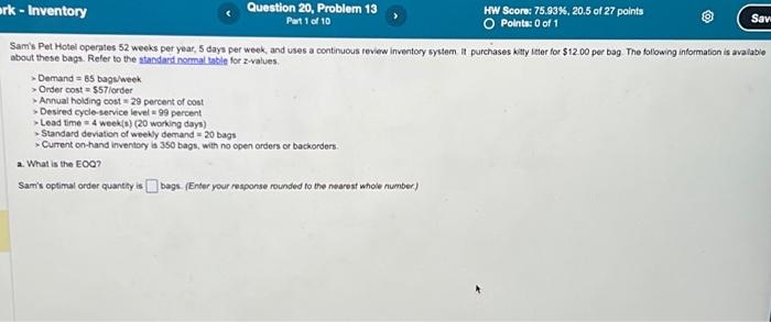
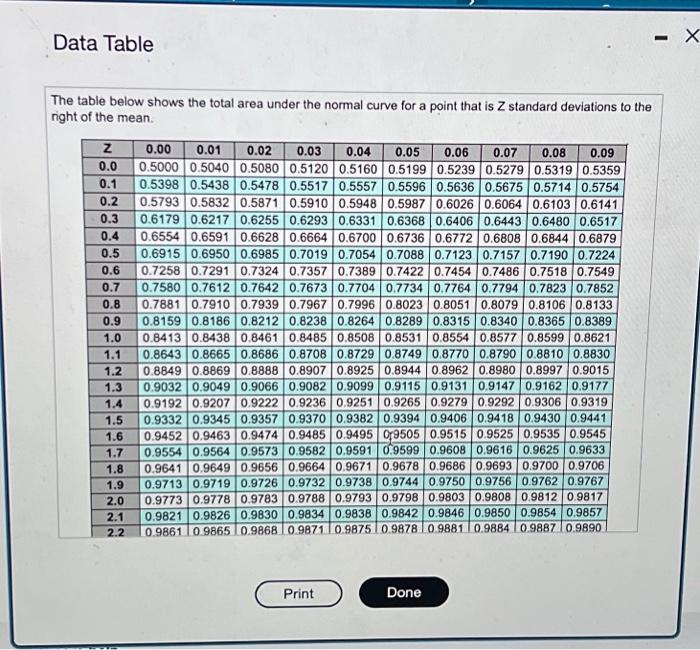
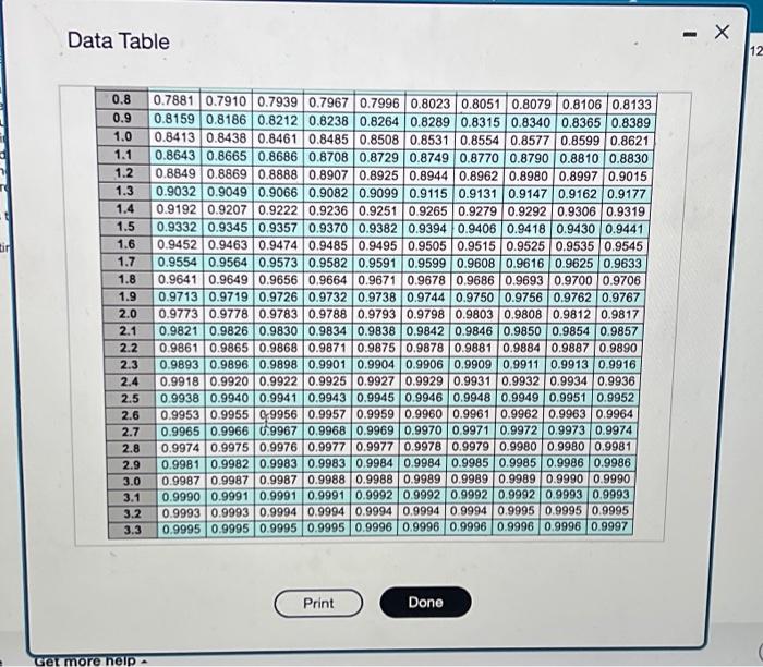
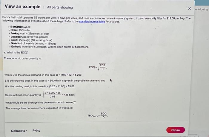
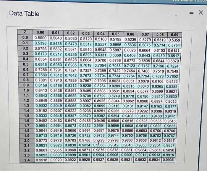
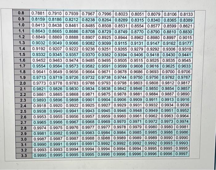
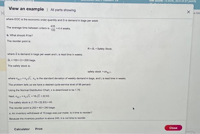
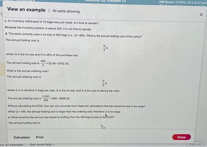
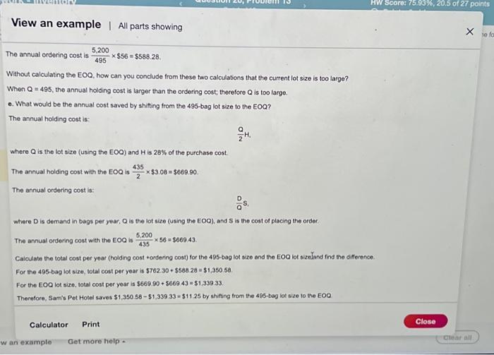
Sam's Pet Hotel operates 52 weeks per year, 5 days per week, and uses a continuous review inventory system. It purchases kitty litter for $11.00 per bag. The following information is avalable about these bags. Refor to the standard normat table for z-values. > Bdeckabs/week > Ontur $56 iorder > Aariag cost =28 percent of cost > Egriereatrvice level =96 percent > tirad =2 week(s) ( 10 working days) > Skenctiod of weekly demand =16 bags > Qstent imventory is 310 bags, with no open orders or backorders. a. What is the EOQ? The economic order quantity is: EOQ=H2DS where D is the annual demand, in this case D=(10052)=5,200, S is the ordering cost, in this case S=56, which is given in the problem statement, and H is the holding cost, in this case H=(0.2811.00)=$3.08. Sam's optimal order quantity is 3.0025,20056=435 bags. What would be the average time between orders (in weeks)? The average time between orders, expressed in weeks, is: TBOEOO=DEOO The annual ordering cost is 4955,200$56=$588.28, Without calculating the EOQ, how can you conclude from these two calculations that the current lot size is too large? When Q=495, the annual holding cost is larger than the ordering cost; therefore Q is too large. e. What would be the annual cost saved by shifting from the 495 -bag lot size to the EOQ? The annual holding cost is: 2QH4 where Q is the lot size (using the EOO) and H is 28% of the purchase cost. The annual holding cost with the EOQ is 2435$3.08=$669.90 The annual ordering cost is: QDS Where D is demand in bags per year, Q is the lot size (Using the EOO), and S is the cost of placing the order. The annual ordering cost with the EOQ is 4355,20056=$669.43. Calculate the total cost per year (holding cost +ordering cost) for the 495.bag lot size and the EOO lot sizeland find the differen For the 495-bag lot size, total cost per year is $762.30+$580.28=$1,350.5a. For the EOO lot size, total cost per year is $669.90+$669.43=$1,339.33. Thernfore, Sam's Pet Hotel saves $1,350.58$1,339.33=$11.25 by shifting trom the 495 bag lot size to the EOO Data Table Samis Pet Hotel operates 52 weeks per year, 5 days per week, and uses a continuous teview inventory system. it purchases kitty leter for $12.00 per bag . The following information is avalable about these bags. Refler to the standard nomal tabile for z-values. > Demand =85 bagelweek > Onder cost =$57 lorder > Annual holding cost = 29 percent of cost - Desired cycle-service levet =99 percent - Lead time =4 week (s) (20 working days) - Standard deviation of weekly demand =20 bags > Current on hand inventory is 350 bags, with no open orders or backorders. a. What is the EOO? Sam's optimal order quantify is bags. (Enter your response rounded to the nearest whole number) where EOC is the economic order quantity and D is demand in bags per week. The average time between orders is 100435=4.4 weeks. b. What should R be? The reorder point is: R=d~L+SafetyStock Where d is demand in bags per week and L is lead time in weeks. dL=1002=200bags. The safety stock is: safetystock=20dLT. where dLT=dL,d is the standard deviation of weekly demand in bags, and L is lead time in weeks. The problem tells us we have a desired cycle-service level of 96 percent. Using the Normal Distribution Chart, z is determined to be 1.75 Next, dLT=dL=162=22.63. The safety stock is (1.7522.63)=40. The reorder point is 200+40=240 bags c. An inventory withdrawal of 10 bags was just made. Is it time to reorden Because the inventory position is abeve 240 , it is not time to reordet. Data Table The table below shows the total area under the normal curve for a point that is Z standard deviations to the ight of the mean. c. An inventory withdrawal of 10 bags was just made. Is it time to reorder? Because the inventory position is above 240 , it is not time to reorder. d. The store currently uses a lot size of 495 bags (i.e, Q=495 ). What is the annual holding cost of this policy? The annual hoiding cost is: 2QH Where Q is the lot size and H is 2A% of the purchase cost. The annual holding cost is 2495$3.08=$762.30. What is the annual ordering cost? The annual ordering cost is: ODS Where D is is demand in bags per year, Q is the lot size, and S is the cost of placing the order. The annual ordering cost is 4955.200$56=$588.28. Without calculating the EOO, how can you conclude from these two calculations that the current lot size is too large? When Q=495, the annual holding cost is larger than the ordering cost; therefore Q is too large. e. What would be the annual cost saved by shifting from the 495 -bag lot size to the "EOQ? The annual hoiding cost is: QH \begin{tabular}{|c|c|c|c|c|c|c|c|c|c|c|} \hline 0.8 & 0.7881 & 0.7910 & 0.7939 & 0.7967 & 0.7996 & 0.8023 & 0.8051 & 0.8079 & 0.8106 & 0.8133 \\ \hline 0.9 & 0.8159 & 0.8186 & 0.8212 & 0.8238 & 0.8264 & 0.8289 & 0.8315 & 0.8340 & 0.8365 & 0.8389 \\ \hline 1.0 & 0.8413 & 0.8438 & 0.8461 & 0.8485 & 0.8508 & 0.8531 & 0.8554 & 0.8577 & 0.8599 & 0.8621 \\ \hline 1.1 & 0.8643 & 0.8665 & 0.8686 & 0.8708 & 0.8729 & 0.8749 & 0.8770 & 0.8790 & 0.8810 & 0.8830 \\ \hline 1.2 & 0.8849 & 0.8869 & 0.8888 & 0.8907 & 0.8925 & 0.8944 & 0.8962 & 0.8980 & 0.8997 & 0.9015 \\ \hline 1.3 & 0.9032 & 0.9049 & 0.9066 & 0.9082 & 0.9099 & 0.9115 & 0.9131 & 0.9147 & \begin{tabular}{|l|l|} 0.9162 \\ \end{tabular} & 0.9177 \\ \hline 1.4 & 0.9192 & 0.9207 & 0.9222 & 0.9236 & 0.9251 & 0.9265 & 0.9279 & 0.9292 & 0.9306 & 0.9319 \\ \hline 1.5 & 0.9332 & 0.9345 & 0.9357 & 0.9370 & 0.9382 & 0.9394 & 0.9406 & 0.9418 & 0.9430 & 0.9441 \\ \hline 1.6 & 0.9452 & 0.9463 & 0.9474 & 0.9485 & 0.9495 & 0.9505 & 0.9515 & 0.9525 & 0.9535 & 0.9545 \\ \hline 1.7 & 0.9554 & 0.9564 & 0.9573 & 0.9582 & 0.9591 & 0.9599 & 0.9608 & 0.9616 & 0.9625 & 0.9633 \\ \hline 1.8 & 0.9641 & 0.9649 & 0.9656 & 0.9664 & 0.9671 & 0.9678 & \begin{tabular}{|l|} 0.9686 \\ \end{tabular} & 0.9693 & 0.9700 & 0.9706 \\ \hline 1.9 & 0.9713 & 0.9719 & 0.9726 & 0.9732 & 0.9738 & 0.9744 & 0.9750 & 0.9756 & 0.9762 & 0.9767 \\ \hline 2.0 & 0.9773 & 0.9778 & 0.9783 & 0.9788 & 0.9793 & 0.9798 & 0.9803 & 0.9808 & 0.9812 & 0.9817 \\ \hline 2.1 & 0.9821 & 0.9826 & 0.9830 & 0.9834 & 0.9838 & 0.9842 & 0.9846 & 0.9850 & 0.9854 & 0.9857 \\ \hline 2.2 & 0.9861 & 0.9865 & 0.9868 & 0.9871 & 0.9875 & 0.9878 & 0.9881 & 0.9884 & 0.9887 & 0.9890 \\ \hline 2.3 & 0.9893 & 0.9896 & 0.9898 & 0.9901 & 0.9904 & 0.9906 & 0.9909 & 0.9911 & 0.9913 & 0.9916 \\ \hline 2.4 & 0.9918 & 0.9920 & 0.9922 & 0.9925 & \begin{tabular}{|l|} 0.9927 \\ \end{tabular} & 0.9929 & 0.9931 & 0.9932 & 0.9934 & 0.9936 \\ \hline 2.5 & 0.9938 & 0.9940 & 0.9941 & 0.9943 & 0.9945 & 0.9946 & 0.9948 & 0.9949 & 0.9951 & 0.9952 \\ \hline 2.6 & 0.9953 & 0.9955 & 0.9956 & 0.9957 & 0.9959 & 0.9960 & 0.9961 & 0.9962 & 0.9963 & 0.9964 \\ \hline 2.7 & 0.9965 & 0.9966 & 0.9967 & 0.9968 & 0.9969 & 0.9970 & 0.9971 & 0.9972 & 0.9973 & 0.9974 \\ \hline 2.8 & 0.9974 & 0.9975 & 0.9976 & 0.9977 & 0.9977 & 0.9978 & 0.9979 & 0.9980 & 0.9980 & 0.9981 \\ \hline 2.9 & \begin{tabular}{|l|l|} 0.9981 \\ \end{tabular} & 0.9982 & 0.9983 & 0.9983 & 0.9984 & 0.9984 & 0.9985 & 0.9985 & 0.9986 & 0.9986 \\ \hline 3.0 & 0.9987 & \begin{tabular}{|c|} 0.9987 \\ \end{tabular} & 0.9987 & 0.9988 & 0.9688 & 0.9989 & 0.9989 & 0.9989 & 0.9990 & 0.9990 \\ \hline 3.1 & 0.9990 & 0.9991 & 0.9991 & 0.9991 & 0.9992 & 0.9992 & 0.9992 & 0.9992 & 0.9993 & 0.9993 \\ \hline 3.2 & 0.9993 & 0.9993 & 0.9994 & 0.9994 & 0.9994 & 0.9994 & 0.9994 & 0.9995 & 0.9995 & 0.9995 \\ \hline 3.3 & 0.9995 & 0.9995 & 0.9995 & 0.9995 & 0.9996 & 0.9996 & 0.9996 & 0.9996 & 0.9996 & 0.9997 \\ \hline \end{tabular} Sam's Pet Hotel operates 52 weeks per year, 5 days per week, and uses a continuous review inventory system. It purchases kitty litter for $11.00 per bag. The following information is avalable about these bags. Refor to the standard normat table for z-values. > Bdeckabs/week > Ontur $56 iorder > Aariag cost =28 percent of cost > Egriereatrvice level =96 percent > tirad =2 week(s) ( 10 working days) > Skenctiod of weekly demand =16 bags > Qstent imventory is 310 bags, with no open orders or backorders. a. What is the EOQ? The economic order quantity is: EOQ=H2DS where D is the annual demand, in this case D=(10052)=5,200, S is the ordering cost, in this case S=56, which is given in the problem statement, and H is the holding cost, in this case H=(0.2811.00)=$3.08. Sam's optimal order quantity is 3.0025,20056=435 bags. What would be the average time between orders (in weeks)? The average time between orders, expressed in weeks, is: TBOEOO=DEOO The annual ordering cost is 4955,200$56=$588.28, Without calculating the EOQ, how can you conclude from these two calculations that the current lot size is too large? When Q=495, the annual holding cost is larger than the ordering cost; therefore Q is too large. e. What would be the annual cost saved by shifting from the 495 -bag lot size to the EOQ? The annual holding cost is: 2QH4 where Q is the lot size (using the EOO) and H is 28% of the purchase cost. The annual holding cost with the EOQ is 2435$3.08=$669.90 The annual ordering cost is: QDS Where D is demand in bags per year, Q is the lot size (Using the EOO), and S is the cost of placing the order. The annual ordering cost with the EOQ is 4355,20056=$669.43. Calculate the total cost per year (holding cost +ordering cost) for the 495.bag lot size and the EOO lot sizeland find the differen For the 495-bag lot size, total cost per year is $762.30+$580.28=$1,350.5a. For the EOO lot size, total cost per year is $669.90+$669.43=$1,339.33. Thernfore, Sam's Pet Hotel saves $1,350.58$1,339.33=$11.25 by shifting trom the 495 bag lot size to the EOO Data Table Samis Pet Hotel operates 52 weeks per year, 5 days per week, and uses a continuous teview inventory system. it purchases kitty leter for $12.00 per bag . The following information is avalable about these bags. Refler to the standard nomal tabile for z-values. > Demand =85 bagelweek > Onder cost =$57 lorder > Annual holding cost = 29 percent of cost - Desired cycle-service levet =99 percent - Lead time =4 week (s) (20 working days) - Standard deviation of weekly demand =20 bags > Current on hand inventory is 350 bags, with no open orders or backorders. a. What is the EOO? Sam's optimal order quantify is bags. (Enter your response rounded to the nearest whole number) where EOC is the economic order quantity and D is demand in bags per week. The average time between orders is 100435=4.4 weeks. b. What should R be? The reorder point is: R=d~L+SafetyStock Where d is demand in bags per week and L is lead time in weeks. dL=1002=200bags. The safety stock is: safetystock=20dLT. where dLT=dL,d is the standard deviation of weekly demand in bags, and L is lead time in weeks. The problem tells us we have a desired cycle-service level of 96 percent. Using the Normal Distribution Chart, z is determined to be 1.75 Next, dLT=dL=162=22.63. The safety stock is (1.7522.63)=40. The reorder point is 200+40=240 bags c. An inventory withdrawal of 10 bags was just made. Is it time to reorden Because the inventory position is abeve 240 , it is not time to reordet. Data Table The table below shows the total area under the normal curve for a point that is Z standard deviations to the ight of the mean. c. An inventory withdrawal of 10 bags was just made. Is it time to reorder? Because the inventory position is above 240 , it is not time to reorder. d. The store currently uses a lot size of 495 bags (i.e, Q=495 ). What is the annual holding cost of this policy? The annual hoiding cost is: 2QH Where Q is the lot size and H is 2A% of the purchase cost. The annual holding cost is 2495$3.08=$762.30. What is the annual ordering cost? The annual ordering cost is: ODS Where D is is demand in bags per year, Q is the lot size, and S is the cost of placing the order. The annual ordering cost is 4955.200$56=$588.28. Without calculating the EOO, how can you conclude from these two calculations that the current lot size is too large? When Q=495, the annual holding cost is larger than the ordering cost; therefore Q is too large. e. What would be the annual cost saved by shifting from the 495 -bag lot size to the "EOQ? The annual hoiding cost is: QH \begin{tabular}{|c|c|c|c|c|c|c|c|c|c|c|} \hline 0.8 & 0.7881 & 0.7910 & 0.7939 & 0.7967 & 0.7996 & 0.8023 & 0.8051 & 0.8079 & 0.8106 & 0.8133 \\ \hline 0.9 & 0.8159 & 0.8186 & 0.8212 & 0.8238 & 0.8264 & 0.8289 & 0.8315 & 0.8340 & 0.8365 & 0.8389 \\ \hline 1.0 & 0.8413 & 0.8438 & 0.8461 & 0.8485 & 0.8508 & 0.8531 & 0.8554 & 0.8577 & 0.8599 & 0.8621 \\ \hline 1.1 & 0.8643 & 0.8665 & 0.8686 & 0.8708 & 0.8729 & 0.8749 & 0.8770 & 0.8790 & 0.8810 & 0.8830 \\ \hline 1.2 & 0.8849 & 0.8869 & 0.8888 & 0.8907 & 0.8925 & 0.8944 & 0.8962 & 0.8980 & 0.8997 & 0.9015 \\ \hline 1.3 & 0.9032 & 0.9049 & 0.9066 & 0.9082 & 0.9099 & 0.9115 & 0.9131 & 0.9147 & \begin{tabular}{|l|l|} 0.9162 \\ \end{tabular} & 0.9177 \\ \hline 1.4 & 0.9192 & 0.9207 & 0.9222 & 0.9236 & 0.9251 & 0.9265 & 0.9279 & 0.9292 & 0.9306 & 0.9319 \\ \hline 1.5 & 0.9332 & 0.9345 & 0.9357 & 0.9370 & 0.9382 & 0.9394 & 0.9406 & 0.9418 & 0.9430 & 0.9441 \\ \hline 1.6 & 0.9452 & 0.9463 & 0.9474 & 0.9485 & 0.9495 & 0.9505 & 0.9515 & 0.9525 & 0.9535 & 0.9545 \\ \hline 1.7 & 0.9554 & 0.9564 & 0.9573 & 0.9582 & 0.9591 & 0.9599 & 0.9608 & 0.9616 & 0.9625 & 0.9633 \\ \hline 1.8 & 0.9641 & 0.9649 & 0.9656 & 0.9664 & 0.9671 & 0.9678 & \begin{tabular}{|l|} 0.9686 \\ \end{tabular} & 0.9693 & 0.9700 & 0.9706 \\ \hline 1.9 & 0.9713 & 0.9719 & 0.9726 & 0.9732 & 0.9738 & 0.9744 & 0.9750 & 0.9756 & 0.9762 & 0.9767 \\ \hline 2.0 & 0.9773 & 0.9778 & 0.9783 & 0.9788 & 0.9793 & 0.9798 & 0.9803 & 0.9808 & 0.9812 & 0.9817 \\ \hline 2.1 & 0.9821 & 0.9826 & 0.9830 & 0.9834 & 0.9838 & 0.9842 & 0.9846 & 0.9850 & 0.9854 & 0.9857 \\ \hline 2.2 & 0.9861 & 0.9865 & 0.9868 & 0.9871 & 0.9875 & 0.9878 & 0.9881 & 0.9884 & 0.9887 & 0.9890 \\ \hline 2.3 & 0.9893 & 0.9896 & 0.9898 & 0.9901 & 0.9904 & 0.9906 & 0.9909 & 0.9911 & 0.9913 & 0.9916 \\ \hline 2.4 & 0.9918 & 0.9920 & 0.9922 & 0.9925 & \begin{tabular}{|l|} 0.9927 \\ \end{tabular} & 0.9929 & 0.9931 & 0.9932 & 0.9934 & 0.9936 \\ \hline 2.5 & 0.9938 & 0.9940 & 0.9941 & 0.9943 & 0.9945 & 0.9946 & 0.9948 & 0.9949 & 0.9951 & 0.9952 \\ \hline 2.6 & 0.9953 & 0.9955 & 0.9956 & 0.9957 & 0.9959 & 0.9960 & 0.9961 & 0.9962 & 0.9963 & 0.9964 \\ \hline 2.7 & 0.9965 & 0.9966 & 0.9967 & 0.9968 & 0.9969 & 0.9970 & 0.9971 & 0.9972 & 0.9973 & 0.9974 \\ \hline 2.8 & 0.9974 & 0.9975 & 0.9976 & 0.9977 & 0.9977 & 0.9978 & 0.9979 & 0.9980 & 0.9980 & 0.9981 \\ \hline 2.9 & \begin{tabular}{|l|l|} 0.9981 \\ \end{tabular} & 0.9982 & 0.9983 & 0.9983 & 0.9984 & 0.9984 & 0.9985 & 0.9985 & 0.9986 & 0.9986 \\ \hline 3.0 & 0.9987 & \begin{tabular}{|c|} 0.9987 \\ \end{tabular} & 0.9987 & 0.9988 & 0.9688 & 0.9989 & 0.9989 & 0.9989 & 0.9990 & 0.9990 \\ \hline 3.1 & 0.9990 & 0.9991 & 0.9991 & 0.9991 & 0.9992 & 0.9992 & 0.9992 & 0.9992 & 0.9993 & 0.9993 \\ \hline 3.2 & 0.9993 & 0.9993 & 0.9994 & 0.9994 & 0.9994 & 0.9994 & 0.9994 & 0.9995 & 0.9995 & 0.9995 \\ \hline 3.3 & 0.9995 & 0.9995 & 0.9995 & 0.9995 & 0.9996 & 0.9996 & 0.9996 & 0.9996 & 0.9996 & 0.9997 \\ \hline \end{tabular}
