Excel 2016 module 9 case problem 3 questions 13, 16, 17 and 18

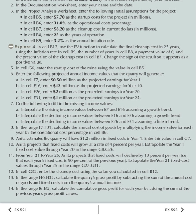
2. In the Documentation worksheet, enter your name and the date. 3. In the Project Analysis worksheet, enter the following initial assumptions for the project: In cell B5, enter $7.70 as the startup costs for the project (in millions). In cell B6, enter 31.0% as the operational costs percentage. In cell B7, enter $8.20 as the cleanup cost in current dollars (in millions). In cell B8, enter 25 as the years of operation. In cell B9, enter 3.2% as the annual inflation rate. Explore 4. In cell B12, use the FV function to calculate the final cleanup cost in 25 years, using the inflation rate in cell B9, the number of years in cell B8, a payment value of 0, and the present value of the cleanup cost in cell B7. Change the sign of the result so it appears as a positive value. 5. In cell G6, enter the startup cost of the mine using the value in cell B5. 6. Enter the following projected annual income values that the quarry will generate: a. In cell E7, enter $0.50 million as the projected earnings for Year 1. b. In cell E16, enter $12 million as the projected earnings for Year 10. c. In cell E26, enter $2 million as the projected earnings for Year 20. d. In cell E31, enter $1 million as the projected earnings for Year 25. 7. Do the following to fill in the missing income values: a. Interpolate the rising income values between E7 and E16 assuming a growth trend. b. Interpolate the declining income values between E16 and E26 assuming a growth trend. c. Interpolate the declining income values between E26 and E31 assuming a linear trend. 8. In the range F7:F31, calculate the annual cost of goods by multiplying the income value for each year by the operational cost percentage in cell B6. 9. Anita estimates the quarry will have $1.2 million in fixed costs in Year 1. Enter this value in cell G7. 10. Anita projects that fixed costs will grow at a rate of 4 percent per year. Extrapolate the Year 1 fixed cost value through Year 20 in the range G8:G26. 11. From Year 21 to Year 25, Anita projects that fixed costs will decline by 10 percent per year (so that each year's fixed cost is 90 percent of the previous year). Extrapolate the Year 21 fixed-cost values through Year 25 in the range G27:G31. 12. In cell G32, enter the cleanup cost using the value you calculated in cell B12. 13. In the range 16:H32, calculate the quarry's gross profit by subtracting the sum of the annual cost of goods and fixed costs from the quarry's annual income. 14. In the range 16:132, calculate the cumulative gross profit for each year by adding the sum of the previous year's gross profit values. 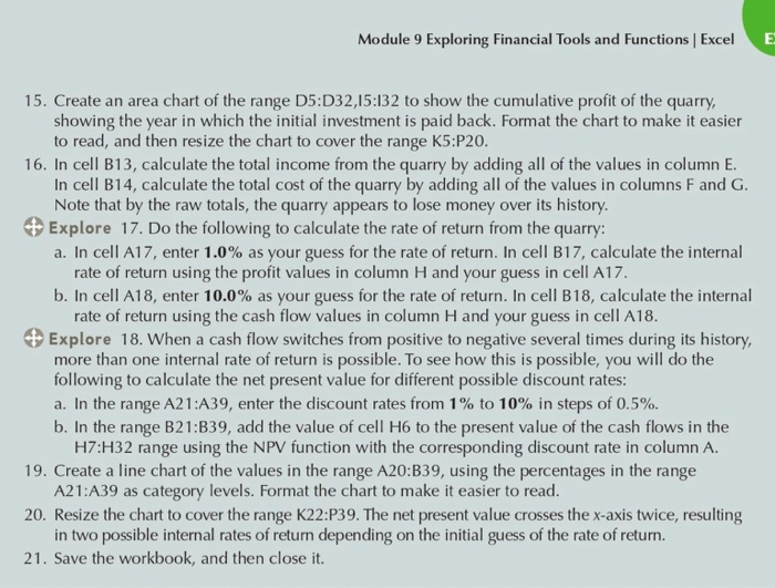Module 9 Exploring Financial Tools and Functions | Excel E 15. Create an area chart of the range D5:D32,15:132 to show the cumulative profit of the quarry, showing the year in which the initial investment is paid back. Format the chart to make it easier to read, and then resize the chart to cover the range K5:P20. 16. In cell B13, calculate the total income from the quarry by adding all of the values in column E. In cell B14, calculate the total cost of the quarry by adding all of the values in columns F and G. Note that by the raw totals, the quarry appears to lose money over its history. Explore 17. Do the following to calculate the rate of return from the quarry: a. In cell A17, enter 1.0% as your guess for the rate of return. In cell B17, calculate the internal rate of return using the profit values in column H and your guess in cell A17. b. In cell A18, enter 10.0% as your guess for the rate of return. In cell B18, calculate the internal rate of return using the cash flow values in column H and your guess in cell A18. Explore 18. When a cash flow switches from positive to negative several times during its history, more than one internal rate of return is possible. To see how this is possible, you will do the following to calculate the net present value for different possible discount rates: a. In the range A21:A39, enter the discount rates from 1% to 10% in steps of 0.5%. b. In the range B21:B39, add the value of cell H6 to the present value of the cash flows in the H7:H32 range using the NPV function with the corresponding discount rate in column A. 19. Create a line chart of the values in the range A20:339, using the percentages in the range A21:A39 as category levels. Format the chart to make it easier to read. 20. Resize the chart to cover the range K22:P39. The net present value crosses the x-axis twice, resulting in two possible internal rates of return depending on the initial guess of the rate of return. 21. Save the workbook, and then close it. 2. In the Documentation worksheet, enter your name and the date. 3. In the Project Analysis worksheet, enter the following initial assumptions for the project: In cell B5, enter $7.70 as the startup costs for the project (in millions). In cell B6, enter 31.0% as the operational costs percentage. In cell B7, enter $8.20 as the cleanup cost in current dollars (in millions). In cell B8, enter 25 as the years of operation. In cell B9, enter 3.2% as the annual inflation rate. Explore 4. In cell B12, use the FV function to calculate the final cleanup cost in 25 years, using the inflation rate in cell B9, the number of years in cell B8, a payment value of 0, and the present value of the cleanup cost in cell B7. Change the sign of the result so it appears as a positive value. 5. In cell G6, enter the startup cost of the mine using the value in cell B5. 6. Enter the following projected annual income values that the quarry will generate: a. In cell E7, enter $0.50 million as the projected earnings for Year 1. b. In cell E16, enter $12 million as the projected earnings for Year 10. c. In cell E26, enter $2 million as the projected earnings for Year 20. d. In cell E31, enter $1 million as the projected earnings for Year 25. 7. Do the following to fill in the missing income values: a. Interpolate the rising income values between E7 and E16 assuming a growth trend. b. Interpolate the declining income values between E16 and E26 assuming a growth trend. c. Interpolate the declining income values between E26 and E31 assuming a linear trend. 8. In the range F7:F31, calculate the annual cost of goods by multiplying the income value for each year by the operational cost percentage in cell B6. 9. Anita estimates the quarry will have $1.2 million in fixed costs in Year 1. Enter this value in cell G7. 10. Anita projects that fixed costs will grow at a rate of 4 percent per year. Extrapolate the Year 1 fixed cost value through Year 20 in the range G8:G26. 11. From Year 21 to Year 25, Anita projects that fixed costs will decline by 10 percent per year (so that each year's fixed cost is 90 percent of the previous year). Extrapolate the Year 21 fixed-cost values through Year 25 in the range G27:G31. 12. In cell G32, enter the cleanup cost using the value you calculated in cell B12. 13. In the range 16:H32, calculate the quarry's gross profit by subtracting the sum of the annual cost of goods and fixed costs from the quarry's annual income. 14. In the range 16:132, calculate the cumulative gross profit for each year by adding the sum of the previous year's gross profit values. Module 9 Exploring Financial Tools and Functions | Excel E 15. Create an area chart of the range D5:D32,15:132 to show the cumulative profit of the quarry, showing the year in which the initial investment is paid back. Format the chart to make it easier to read, and then resize the chart to cover the range K5:P20. 16. In cell B13, calculate the total income from the quarry by adding all of the values in column E. In cell B14, calculate the total cost of the quarry by adding all of the values in columns F and G. Note that by the raw totals, the quarry appears to lose money over its history. Explore 17. Do the following to calculate the rate of return from the quarry: a. In cell A17, enter 1.0% as your guess for the rate of return. In cell B17, calculate the internal rate of return using the profit values in column H and your guess in cell A17. b. In cell A18, enter 10.0% as your guess for the rate of return. In cell B18, calculate the internal rate of return using the cash flow values in column H and your guess in cell A18. Explore 18. When a cash flow switches from positive to negative several times during its history, more than one internal rate of return is possible. To see how this is possible, you will do the following to calculate the net present value for different possible discount rates: a. In the range A21:A39, enter the discount rates from 1% to 10% in steps of 0.5%. b. In the range B21:B39, add the value of cell H6 to the present value of the cash flows in the H7:H32 range using the NPV function with the corresponding discount rate in column A. 19. Create a line chart of the values in the range A20:339, using the percentages in the range A21:A39 as category levels. Format the chart to make it easier to read. 20. Resize the chart to cover the range K22:P39. The net present value crosses the x-axis twice, resulting in two possible internal rates of return depending on the initial guess of the rate of return. 21. Save the workbook, and then close it