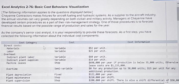
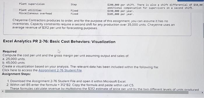
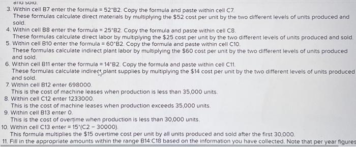
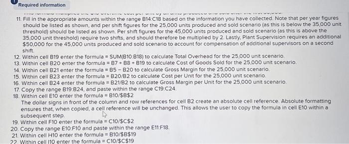
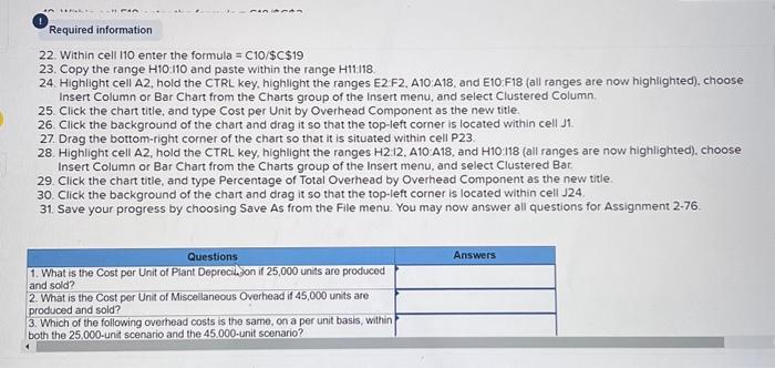
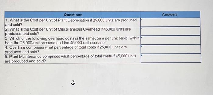
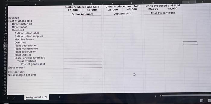
Excel Analytics 2-76: Basic Cost Behaviors: Visualization [The following information applies to the questions displayed below] Cheyenne Contractors makes fixtures for aircraft fueling and hydraulic systems. As a supplier to the aircraft industry. the annual volumes can vary greatly depending on both civilian and military activity. Managers at Cheyenne have developed certain procedures as a part of their risk-management strategy. One of those procedures is to forecast financial results based on the possible range of production and sales for the year. As the company's senior cost analyst, it is your responsibility to provide these forecasts. As a first step, you have collected the following information about the indlididual cost components: Cheyenne Contractors produces to order, and for the purpose of this assignment, you can assume it has no inventories. Capacity constraints require a second shift for any production over 35,000 units. Cheyenne uses an average revenue of $312 per unit for forecasting purposes. Excel Analytics PR 2-76: Basic Cost Behaviors: Visualization Required Compute the cost per unit and the gross margin per unit assuming output and sales of: a. 25,000 units. b. 45,000 units Create a visualization based on your analysis. The relevant data has been included within the following file: Click here to access the Assignment 2.76 Student File. Assignment Steps: 1. Downioad the Assignment 2.76 Student File and open it within Microsoft Excel. 2. Within cell B5 enter the formula =312B2. Copy the formula and paste within cell C5. These formulas calculate revenue bv multiolving the $312 estimate of orice ver unit by the two different levels of units oroduced 3. Within cell B7 enter the formula =52B2. Copy the formula and paste within cell C7. These formulas calculate direct materials by multiplying the $52 cost per unit by the two different levels of units produced and sold. 4. Within cell B8 enter the formula =25B2. Copy the formula and paste within cell C8. These formulas calculate direct labor by multiplying the $25 cost per unit by the two different levels of units produced and sold. 5. Within cell B10 enter the formula =60B2. Copy the formula and paste within cell C10 : These formulas calculate indirect plant labor by multiplying the $60 cost per unit by the two different leveis of units produced and sold. 6. Within cell B11 enter the formula =14B2. Copy the formula and paste within cell C11. These formulas calculate indirees plant supplies by multiplying the $14 cost per unit by the two different levels of units produced and sold. 7. Within cell B12 enter 698000 This is the cost of machine leases when production is less than 35,000 units: 8. Within cell C12 enter 1233000 . This is the cost of machine leases when production exceeds 35,000 units 9. Within cell B13 enter O. This is the cost of overtime when production is less than 30,000 units. 10. Within cell C13 enter =15(C230000). This formula multiplies the $15 overtime cost per unit by all units produced and sold after the first 30,000 11. Fill in the appropriate amounts within the range B14 C18 based on the information you have collected. Note that per year figures 11. Fill in the appropriate amounts within the range B14C18 based on the information you have collected. Note that per year figures should be listed as shown, and per shift figures for the 25,000 units produced and sold scenario (as this is below the 35.000 unit threshold) should be listed as shown. Per shift figures for the 45.000 units produced and sold scenario (as this is above the 35,000 unit threshold) require two shifts, and should therefore be multiplied by 2 . Lastly, Plant Supervision requires an additional $50,000 for the 45.000 units produced and sold scenario to account for compensation of additional supervisors on a second shift. 12. Within cell B19 enter the formula =SUM(B10:B18) to calculate Total Overhead for the 25,000 unit scenario 13. Within cell B20 enter the formula =B7+B8+B19 to calculate Cost of Goods Sold for the 25,000 unit scenario 14. Within cell 821 enter the formula = B5 - B20 to calculate Gross Margin for the 25,000 unit scenario. 15. Within cell B23 enter the formula =B20/82 to calculate Cost per Unit for the 25,000 unit scenario. 16. Within cell B24 enter the formula =B21/B2 to calculate Gross Margin per Unit for the 25,000 unit scenario. 17. Copy the range B19:824, and paste within the range C19:C24 18. Within cell E10 enter the formula =B10/$B$2 The dollar signs in front of the column and row references for cell B2 create an absolute cell reference. Absolute formatting ensures that, when copled, a cell reference will be unchanged. This allows the user to copy the formula in cell E10 within a subsequent step. 19. Within cell F10 enter the formula =C1O/$C$2 20. Copy the range E10F10 and paste within the range E11:F18. 21. Within cell HiO enter the formula =B10/$B$19 22. Within cell 110 enter the formula =C10/$c$19 23. Copy the range H10:110 and paste within the range H11:118. 24. Highlight cell A2, hold the CTRL key, highlight the ranges E2F2,A10:A18, and E10:F18 (all ranges are now highlighted), choose Insert Column or Bar Chart from the Charts group of the Insert menu, and select Clustered Column. 25. Click the chart title, and type Cost per Unit by Overhead Component as the new title. 26. Click the background of the chart and drag it so that the top-left corner is located within cell J1. 27. Drag the bottom-right corner of the chart so that it is situated within cell P23. 28. Highlight cell A2, hold the CTRL key, highlight the ranges H212,A10:A18, and H1018 (all ranges are now highighted), choose Insert Column or Bar Chart from the Charts group of the Insert menu, and select Clustered Bar. 29. Click the chart title, and type Percentage of Total Overhead by Overhead Component as the new title. 30. Click the background of the chart and drag it so that the top-left corner is located within cell J24. 31. Save your progress by choosing Save As from the File menu. You may now answer all questions for Assignment 2-76. A. Units Produced and Sold \begin{tabular}{l|l|l|l} H & I & 1 \\ \hline \end{tabular} Units Produced and Sold Units Produced and Sold Units Produced and Sold 25,000 25,000 45,000 25,000 45,000 Dollar Amounts Cost per Unit cost Percentages Revenue Cost of goods sold Direct materials Direct labor Overhead Indirect plant labor indirect plant supplies Machine leases Overtime Plant depreciation Plant maintenance Plant supervision Plant utilities Miscellaneous Overhead Total overhead Cost of goods sold Gross margin Cost per unit Gross margin per unit Assignment 2-76 Excel Analytics 2-76: Basic Cost Behaviors: Visualization [The following information applies to the questions displayed below] Cheyenne Contractors makes fixtures for aircraft fueling and hydraulic systems. As a supplier to the aircraft industry. the annual volumes can vary greatly depending on both civilian and military activity. Managers at Cheyenne have developed certain procedures as a part of their risk-management strategy. One of those procedures is to forecast financial results based on the possible range of production and sales for the year. As the company's senior cost analyst, it is your responsibility to provide these forecasts. As a first step, you have collected the following information about the indlididual cost components: Cheyenne Contractors produces to order, and for the purpose of this assignment, you can assume it has no inventories. Capacity constraints require a second shift for any production over 35,000 units. Cheyenne uses an average revenue of $312 per unit for forecasting purposes. Excel Analytics PR 2-76: Basic Cost Behaviors: Visualization Required Compute the cost per unit and the gross margin per unit assuming output and sales of: a. 25,000 units. b. 45,000 units Create a visualization based on your analysis. The relevant data has been included within the following file: Click here to access the Assignment 2.76 Student File. Assignment Steps: 1. Downioad the Assignment 2.76 Student File and open it within Microsoft Excel. 2. Within cell B5 enter the formula =312B2. Copy the formula and paste within cell C5. These formulas calculate revenue bv multiolving the $312 estimate of orice ver unit by the two different levels of units oroduced 3. Within cell B7 enter the formula =52B2. Copy the formula and paste within cell C7. These formulas calculate direct materials by multiplying the $52 cost per unit by the two different levels of units produced and sold. 4. Within cell B8 enter the formula =25B2. Copy the formula and paste within cell C8. These formulas calculate direct labor by multiplying the $25 cost per unit by the two different levels of units produced and sold. 5. Within cell B10 enter the formula =60B2. Copy the formula and paste within cell C10 : These formulas calculate indirect plant labor by multiplying the $60 cost per unit by the two different leveis of units produced and sold. 6. Within cell B11 enter the formula =14B2. Copy the formula and paste within cell C11. These formulas calculate indirees plant supplies by multiplying the $14 cost per unit by the two different levels of units produced and sold. 7. Within cell B12 enter 698000 This is the cost of machine leases when production is less than 35,000 units: 8. Within cell C12 enter 1233000 . This is the cost of machine leases when production exceeds 35,000 units 9. Within cell B13 enter O. This is the cost of overtime when production is less than 30,000 units. 10. Within cell C13 enter =15(C230000). This formula multiplies the $15 overtime cost per unit by all units produced and sold after the first 30,000 11. Fill in the appropriate amounts within the range B14 C18 based on the information you have collected. Note that per year figures 11. Fill in the appropriate amounts within the range B14C18 based on the information you have collected. Note that per year figures should be listed as shown, and per shift figures for the 25,000 units produced and sold scenario (as this is below the 35.000 unit threshold) should be listed as shown. Per shift figures for the 45.000 units produced and sold scenario (as this is above the 35,000 unit threshold) require two shifts, and should therefore be multiplied by 2 . Lastly, Plant Supervision requires an additional $50,000 for the 45.000 units produced and sold scenario to account for compensation of additional supervisors on a second shift. 12. Within cell B19 enter the formula =SUM(B10:B18) to calculate Total Overhead for the 25,000 unit scenario 13. Within cell B20 enter the formula =B7+B8+B19 to calculate Cost of Goods Sold for the 25,000 unit scenario 14. Within cell 821 enter the formula = B5 - B20 to calculate Gross Margin for the 25,000 unit scenario. 15. Within cell B23 enter the formula =B20/82 to calculate Cost per Unit for the 25,000 unit scenario. 16. Within cell B24 enter the formula =B21/B2 to calculate Gross Margin per Unit for the 25,000 unit scenario. 17. Copy the range B19:824, and paste within the range C19:C24 18. Within cell E10 enter the formula =B10/$B$2 The dollar signs in front of the column and row references for cell B2 create an absolute cell reference. Absolute formatting ensures that, when copled, a cell reference will be unchanged. This allows the user to copy the formula in cell E10 within a subsequent step. 19. Within cell F10 enter the formula =C1O/$C$2 20. Copy the range E10F10 and paste within the range E11:F18. 21. Within cell HiO enter the formula =B10/$B$19 22. Within cell 110 enter the formula =C10/$c$19 23. Copy the range H10:110 and paste within the range H11:118. 24. Highlight cell A2, hold the CTRL key, highlight the ranges E2F2,A10:A18, and E10:F18 (all ranges are now highlighted), choose Insert Column or Bar Chart from the Charts group of the Insert menu, and select Clustered Column. 25. Click the chart title, and type Cost per Unit by Overhead Component as the new title. 26. Click the background of the chart and drag it so that the top-left corner is located within cell J1. 27. Drag the bottom-right corner of the chart so that it is situated within cell P23. 28. Highlight cell A2, hold the CTRL key, highlight the ranges H212,A10:A18, and H1018 (all ranges are now highighted), choose Insert Column or Bar Chart from the Charts group of the Insert menu, and select Clustered Bar. 29. Click the chart title, and type Percentage of Total Overhead by Overhead Component as the new title. 30. Click the background of the chart and drag it so that the top-left corner is located within cell J24. 31. Save your progress by choosing Save As from the File menu. You may now answer all questions for Assignment 2-76. A. Units Produced and Sold \begin{tabular}{l|l|l|l} H & I & 1 \\ \hline \end{tabular} Units Produced and Sold Units Produced and Sold Units Produced and Sold 25,000 25,000 45,000 25,000 45,000 Dollar Amounts Cost per Unit cost Percentages Revenue Cost of goods sold Direct materials Direct labor Overhead Indirect plant labor indirect plant supplies Machine leases Overtime Plant depreciation Plant maintenance Plant supervision Plant utilities Miscellaneous Overhead Total overhead Cost of goods sold Gross margin Cost per unit Gross margin per unit Assignment 2-76
