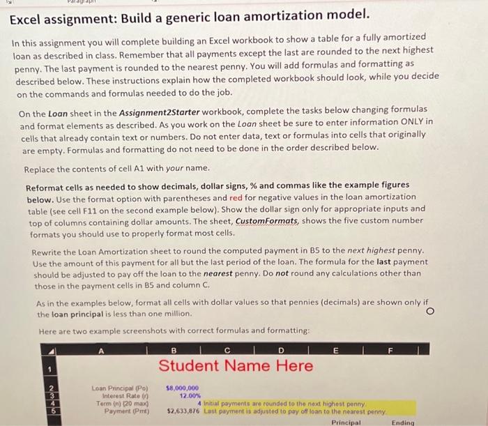
Excel assignment: Build a generic loan amortization model. In this assignment you will complete building an Excel workbook to show a table for a fully amortized loan as described in class. Remember that all payments except the last are rounded to the next highest penny. The last payment is rounded to the nearest penny. You will add formulas and formatting as described below. These instructions explain how the completed workbook should look, while you decide on the commands and formulas needed to do the job. On the Loan sheet in the Assignment2Starter workbook, complete the tasks below changing formulas and format elements as described. As you work on the Loan sheet be sure to enter information ONLY in cells that already contain text or numbers. Do not enter data, text or formulas into cells that originally are empty. Formulas and formatting do not need to be done in the order described below. Replace the contents of cell A1 with your name. Reformat cells as needed to show decimals, dollar signs, % and commas like the example figures below. Use the format option with parentheses and red for negative values in the loan amortization table (see cell F11 on the second example below). Show the dollar sign only for appropriate inputs and top of columns containing dollar amounts. The sheet, CustomFormats, shows the five custom number formats you should use to properly format most cells. Rewrite the Loan Amortization sheet to round the computed payment in B5 to the next highest penny. Use the amount of this payment for all but the last period of the loan. The formula for the last payment should be adjusted to pay off the loan to the nearest penny. Do not round any calculations other than those in the payment cells in B5 and column C. As in the examples below, format all cells with dollar values so that pennies (decimals) are shown only if the loan principal is less than one million. Here are two example screenshots with correct formulas and formatting: 1 2345 A Loan Principal (Po) Interest Rate (r) Term (n) (20 max} Payment (Pmt) B C $8,000,000 12.00% D Student Name Here E 4 Initial payments are rounded to the next highest penny. $2,633,876 Last payment is adjusted to pay off loan to the nearest penny. Principal F Ending


xcel assignment: Build a generic loan amortization model. this assignment you will complete building an Excel workbook to show a table for a fully amortized pan as described in class. Remember that all payments except the last are rounded to the next highest venny. The last payment is rounded to the nearest penny. You will add formulas and formatting as described below. These instructions explain how the completed workbook should look, while you decide on the commands and formulas needed to do the job. On the Loan sheet in the Assignment2Starter workbook, complete the tasks below changing formulas and format elements as described. As you work on the Loan sheet be sure to enter information ONLY in cells that already contain text or numbers. Do not enter data, text or formulas into cells that originally are empty. Formulas and formatting do not need to be done in the order described below. Replace the contents of cell A1 with your name. Reformat cells as needed to show decimals, dollar signs, \% and commas like the example figures below. Use the format option with parentheses and red for negative values in the loan amortization table (see cell F11 on the second example below). Show the dollar sign only for appropriate inputs and top of columns containing dollar amounts. The sheet, Customformats, shows the five custom number formats you should use to properly format most cells. Rewrite the Loan Amortization sheet to round the computed payment in B5 to the next highest penny. Use the amount of this payment for all but the last period of the loan. The formula for the last payment should be adjusted to pay off the loan to the nearest penny. Do not round any calculations other than those in the payment cells in BS and column C. As in the examples below, format all cells with dollar values so that pennies (decimals) are shown only if the loan principal is less than one million. Here are two example screenshots with correct formulas and formatting: Student Name Here Set up the three blue font input cells to accept only reasonable values and prompt with appropriate messages of your choice. For example, none of the inputs should be negative. Constrain term to a whole number between 1 and 20. For each of the three inputs apply appropriate Settings, Input Message and Error Alert using Data Validation on the Data tab in the Ribbon. When the workbook is completed, rows beyond the loan term should look blank on your screen. For example, if the term is set to 10 then rows for periods 11-20 should not be visible, i.e., "blanked out". Devise a way to accomplish this using the IF function with "in ( 2 double quotes) for "blanked out" cells and the ROW function to calculate the End of Period) cell value. There are other ways of accomplishing this, so be sure to use only this method for displaying "blanked out" cell contents. (Do not use conditional formatting to "blank out" rows or use a custom number format (ex. "\#..." or similar) to blank out cells in the workbook. Set up the workbook so that only the input cells may be selected and changed by the user to produce a completed loan amortization table. When finished, be sure to remove any unnecessary conditional formats and reset the values of the three input cells to the original values in the Starter workbook. When finished, zoom the Loan sheet to show approximately cells A1.G31, select cell B2, then Save the workbook. xcel assignment: Build a generic loan amortization model. this assignment you will complete building an Excel workbook to show a table for a fully amortized pan as described in class. Remember that all payments except the last are rounded to the next highest venny. The last payment is rounded to the nearest penny. You will add formulas and formatting as described below. These instructions explain how the completed workbook should look, while you decide on the commands and formulas needed to do the job. On the Loan sheet in the Assignment2Starter workbook, complete the tasks below changing formulas and format elements as described. As you work on the Loan sheet be sure to enter information ONLY in cells that already contain text or numbers. Do not enter data, text or formulas into cells that originally are empty. Formulas and formatting do not need to be done in the order described below. Replace the contents of cell A1 with your name. Reformat cells as needed to show decimals, dollar signs, \% and commas like the example figures below. Use the format option with parentheses and red for negative values in the loan amortization table (see cell F11 on the second example below). Show the dollar sign only for appropriate inputs and top of columns containing dollar amounts. The sheet, Customformats, shows the five custom number formats you should use to properly format most cells. Rewrite the Loan Amortization sheet to round the computed payment in B5 to the next highest penny. Use the amount of this payment for all but the last period of the loan. The formula for the last payment should be adjusted to pay off the loan to the nearest penny. Do not round any calculations other than those in the payment cells in BS and column C. As in the examples below, format all cells with dollar values so that pennies (decimals) are shown only if the loan principal is less than one million. Here are two example screenshots with correct formulas and formatting: Student Name Here Set up the three blue font input cells to accept only reasonable values and prompt with appropriate messages of your choice. For example, none of the inputs should be negative. Constrain term to a whole number between 1 and 20. For each of the three inputs apply appropriate Settings, Input Message and Error Alert using Data Validation on the Data tab in the Ribbon. When the workbook is completed, rows beyond the loan term should look blank on your screen. For example, if the term is set to 10 then rows for periods 11-20 should not be visible, i.e., "blanked out". Devise a way to accomplish this using the IF function with "in ( 2 double quotes) for "blanked out" cells and the ROW function to calculate the End of Period) cell value. There are other ways of accomplishing this, so be sure to use only this method for displaying "blanked out" cell contents. (Do not use conditional formatting to "blank out" rows or use a custom number format (ex. "\#..." or similar) to blank out cells in the workbook. Set up the workbook so that only the input cells may be selected and changed by the user to produce a completed loan amortization table. When finished, be sure to remove any unnecessary conditional formats and reset the values of the three input cells to the original values in the Starter workbook. When finished, zoom the Loan sheet to show approximately cells A1.G31, select cell B2, then Save the workbook


