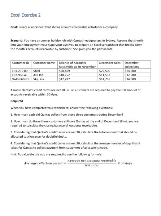
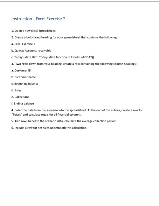
Excel Exercise 2 Goal: Create a worksheet that shows accounts receivable activity for a company. Scenario: You have a summer holiday job with Qantas headquarters in Sydney. Assume that shortly into your employment your supervisor asks you to prepare an Excel spreadsheet that breaks down the month's accounts receivable by customer. She gives you the partial data: Customer ID December sales F01-235-00 FO7-988-45 W40-860-91 Customer name Balance of Accounts Receivable at 30 November Shell $20,469 ADI Ltd $18,752 Sky Link $12,287 $22,500 $11,592 $14,765 December collections $24,500 $12,980 $14,000 Assume Qantas's credit terms are net 30 i.e., all customers are required to pay the full amount of accounts receivable within 30 days. Required When you have completed your worksheet, answer the following questions: 1. How much cash did Qantas collect from these three customers during December? 2. How much do these three customers still owe Qantas at the end of December? (Hint: you are required to calculate the closing balance of Accounts receivable). 3. Considering that Qantas's credit terms are net 30, calculate the total amount that should be allocated to allowance for doubtful debts. 4. Considering that Qantas's credit terms are net 30, calculate the average number of days that it takes for Qantas to collect payment from customers after a sale is made. Hint: To calculate this you are required to use the following formula: Average net accounts receivable Average collection period = Net sales x 30 days Instruction - Excel Exercise 2 1. Open a new Excel Spreadsheet. 2. Create a bold-faced heading for your spreadsheet that contains the following: a. Excel Exercise 2 b. Qantas Accounts receivable C. Today's date Hint: Todays date function in Excel is =TODAY) 3. Two rows down from your heading, create a row containing the following column headings: a. Customer ID b. Customer name C. Beginning balance d. Sales e. Collections f. Ending balance 4. Enter the data from the scenario into the spreadsheet. At the end of the entries, create a row for "Totals" and calculate totals for all financial columns. 5. Two rows beneath the scenario data, calculate the average collection period. 6. Include a row for net sales underneath this calculation