excel help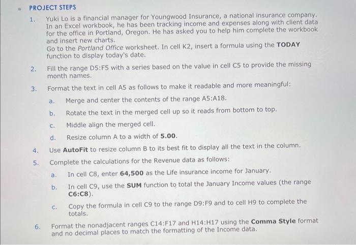

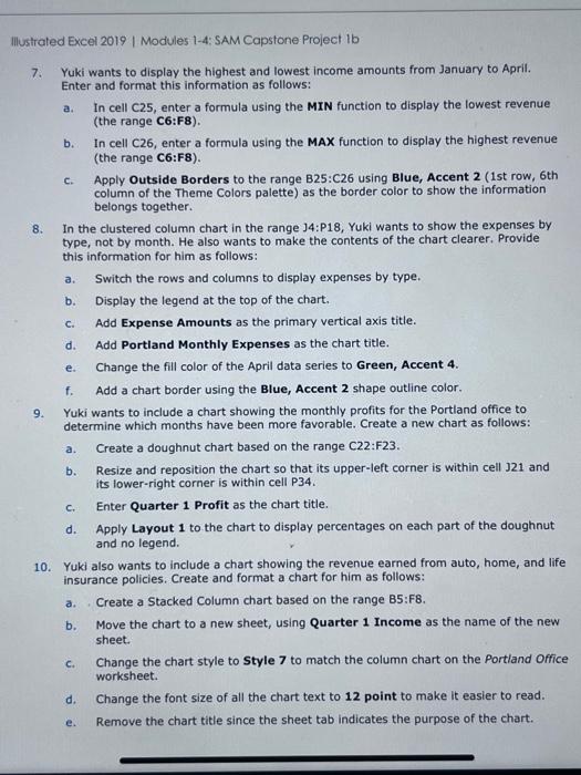
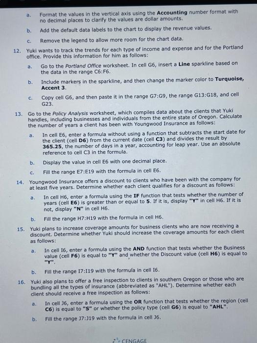
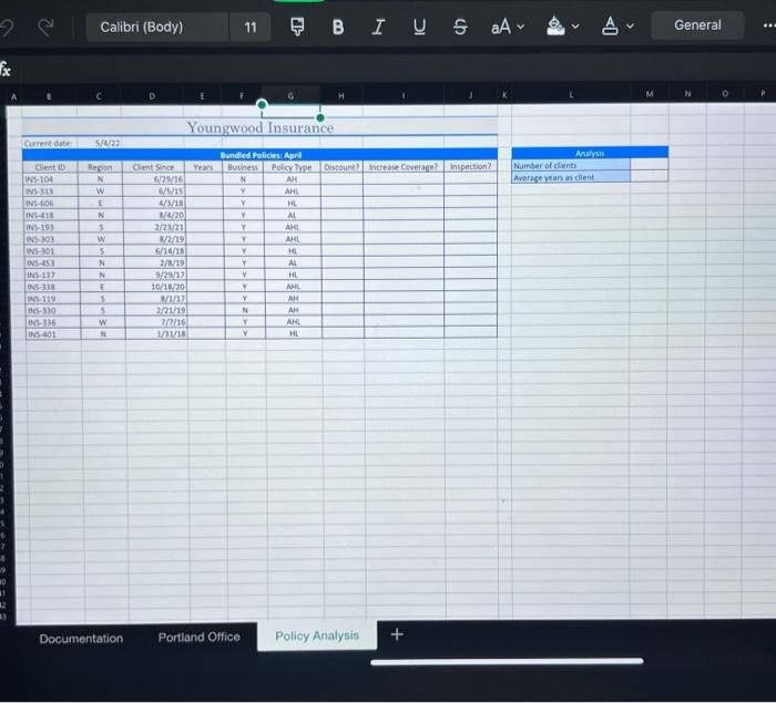
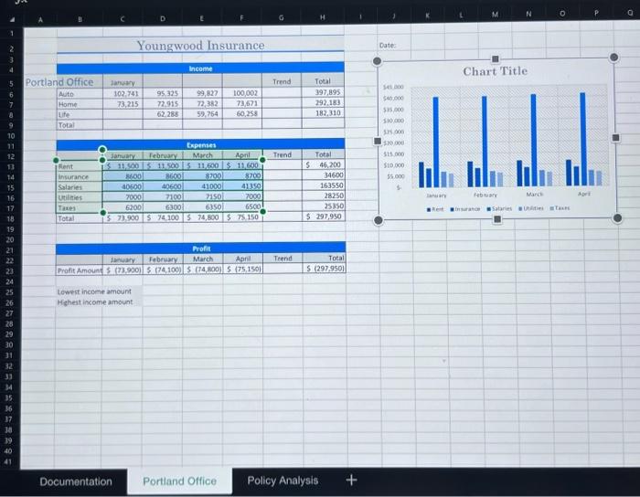
1. Yuki Lo is a financial manager for Youngwood Insurance, a national insurance company. In an Excel workbook, he has been tracking income and expenses along with client data for the office in Portland, Oregon. He has asked you to help him complete the workbook and insert new charts. Go to the Portland Office worksheet. In cell K2, insert a formula using the TODAY function to display today's date. 2. Fill the range D5:F5 with a series based on the value in cell C5 to provide the missing month names. 3. Format the text in cell A5 as follows to make it readable and more meaningful: a. Merge and center the contents of the range A5:A18. b. Rotate the text in the merged cell up so it reads from bottom to top. c. Middle align the merged cell. d. Resize column A to a width of 5.00. 4. Use AutoFit to resize column B to its best fit to display all the text in the column. 5. Complete the calculations for the Revenue data as follows: a. In cell C8, enter 64,500 as the Life insurance income for January. b. In cell C9, use the SUM function to total the January Income values (the range C6:C8). c. Copy the formula in cell C9 to the range D9:F9 and to cell H9 to complete the totals. Illustrated Excel 2019 | Modules 1-4: SAM Capstone Project ib 7. Yuki wants to display the highest and lowest income amounts from January to April. Enter and format this information as follows: a. In cell C25, enter a formula using the MIN function to display the lowest revenue (the range C6:F8 ). b. In cell C26, enter a formula using the MAX function to display the highest revenue (the range C6:F8 ). c. Apply Outside Borders to the range B25:C26 using Blue, Accent 2 (1st row, 6th column of the Theme Colors palette) as the border color to show the information belongs together. 8. In the clustered column chart in the range J4:P18, Yuki wants to show the expenses by type, not by month. He also wants to make the contents of the chart clearer. Provide this information for him as follows: a. Switch the rows and columns to display expenses by type. b. Display the legend at the top of the chart. c. Add Expense Amounts as the primary vertical axis title. d. Add Portland Monthly Expenses as the chart title. e. Change the fill color of the April data series to Green, Accent 4. f. Add a chart border using the Blue, Accent 2 shape outline color. 9. Yuki wants to include a chart showing the monthly profits for the Portland office to determine which months have been more favorable. Create a new chart as follows: a. Create a doughnut chart based on the range C22 :F23. b. Resize and reposition the chart so that its upper-left corner is within cell J21 and its lower-right corner is within cell P34. c. Enter Quarter 1 Profit as the chart title. d. Apply Layout 1 to the chart to display percentages on each part of the doughnut and no legend. 10. Yuki also wants to include a chart showing the revenue earned from auto, home, and life insurance policies. Create and format a chart for him as follows: a. Create a Stacked Column chart based on the range B5:F8. b. Move the chart to a new sheet, using Quarter 1 Income as the name of the new sheet. c. Change the chart style to Style 7 to match the column chart on the Portland Office worksheet. d. Change the font size of all the chart text to 12 point to make it easier to read. e. Remove the chart title since the sheet tab indicates the purpose of the chart. a. Format the values in the vertical axis using the Accounting number format with no decimal places to clarify the values are dollar amounts. b. Add the default data labels to the chart to display the revenue values. c. Remove the legend to allow more room for the chart data. 12. Yuki wants to track the trends for each type of income and expense and for the Portiand office. Provide this information for him as follows: a. Go to the Portland Office worksheet. In cell G6, insert a Line sparkline based on the data in the range C6:F6. b. Include markers in the sparkline, and then change the marker color to Turquoise, Accent 3. c. Copy cell G6, and then paste it in the range G7:G9, the range G13:G18, and cell G23. 13. Go to the Policy Analysis worksheet, which compiles data about the clients that Yuki handies, including businesses and individuals from the entire state of Oregon. Calculate the number of years a client has been with Youngwood Insurance as follows: a. In cell E6, enter a formula without using a function that subtracts the start date for the client (cell D6) from the current date (cell C3) and divides the result by 365.25, the number of days in a year, accounting for leap year. Use an absolute reference to cell C3 in the formula. b. Display the value in cell E6 with one decimal place. c. Fill the range E7:E19 with the formula in cell E6. 14. Youngwood Insurance offers a discount to clients who have been with the company for at least five years. Determine whether each client qualifies for a discount as follows: a. In cell H6, enter a formula using the IF function that tests whether the number of years (cell E6 ) is greater than or equal to 5. If it is, display "Y" in cell H6. If it is not, display " N " in cell H6. b. Fill the range H7:H19 with the formula in cell H6. 15. Yuki plans to increase coverage amounts for business clients who are now receiving a discount. Determine whether Yuki should increase the coverage amounts for each client. as follows: a. In cell 16, enter a formula using the AND function that tests whether the Business value ( cell F6 ) is equal to " Y and whether the Discount value (cell H6 ) is equal to "Y". b. Fill the range 17:119 with the formula in cell 16 . 16. Yuki also plans to offer a free inspection to clients in southern Oregon or those who are bundling all the types of insurance (abbreviated as "AHL"). Determine whether each client should receive a free inspection as follows: a. In cell 36 , enter a formula using the OR function that tests whether the region (cell C6) is equal to " S" or whether the policy type (cell G6) is equal to "AHL". b. Fill the range 37:319 with the formula in cell 36 . A B c. D t. 1 1 M N p Youngwood Insurance Date: Chart Title \begin{tabular}{|c|c|c|c|c|c|r|} \hline \multicolumn{6}{|c|}{ Profit } \\ \hline Femuayy & February & March & April & Teend & Total \\ \hline Profit Amount 5(23,900) & 5(74,100) & 5(74,000) & 5(75,150) & & 5(297,950) \\ \hline \end{tabular} tosest income amount Hghest income amount 1. Yuki Lo is a financial manager for Youngwood Insurance, a national insurance company. In an Excel workbook, he has been tracking income and expenses along with client data for the office in Portland, Oregon. He has asked you to help him complete the workbook and insert new charts. Go to the Portland Office worksheet. In cell K2, insert a formula using the TODAY function to display today's date. 2. Fill the range D5:F5 with a series based on the value in cell C5 to provide the missing month names. 3. Format the text in cell A5 as follows to make it readable and more meaningful: a. Merge and center the contents of the range A5:A18. b. Rotate the text in the merged cell up so it reads from bottom to top. c. Middle align the merged cell. d. Resize column A to a width of 5.00. 4. Use AutoFit to resize column B to its best fit to display all the text in the column. 5. Complete the calculations for the Revenue data as follows: a. In cell C8, enter 64,500 as the Life insurance income for January. b. In cell C9, use the SUM function to total the January Income values (the range C6:C8). c. Copy the formula in cell C9 to the range D9:F9 and to cell H9 to complete the totals. Illustrated Excel 2019 | Modules 1-4: SAM Capstone Project ib 7. Yuki wants to display the highest and lowest income amounts from January to April. Enter and format this information as follows: a. In cell C25, enter a formula using the MIN function to display the lowest revenue (the range C6:F8 ). b. In cell C26, enter a formula using the MAX function to display the highest revenue (the range C6:F8 ). c. Apply Outside Borders to the range B25:C26 using Blue, Accent 2 (1st row, 6th column of the Theme Colors palette) as the border color to show the information belongs together. 8. In the clustered column chart in the range J4:P18, Yuki wants to show the expenses by type, not by month. He also wants to make the contents of the chart clearer. Provide this information for him as follows: a. Switch the rows and columns to display expenses by type. b. Display the legend at the top of the chart. c. Add Expense Amounts as the primary vertical axis title. d. Add Portland Monthly Expenses as the chart title. e. Change the fill color of the April data series to Green, Accent 4. f. Add a chart border using the Blue, Accent 2 shape outline color. 9. Yuki wants to include a chart showing the monthly profits for the Portland office to determine which months have been more favorable. Create a new chart as follows: a. Create a doughnut chart based on the range C22 :F23. b. Resize and reposition the chart so that its upper-left corner is within cell J21 and its lower-right corner is within cell P34. c. Enter Quarter 1 Profit as the chart title. d. Apply Layout 1 to the chart to display percentages on each part of the doughnut and no legend. 10. Yuki also wants to include a chart showing the revenue earned from auto, home, and life insurance policies. Create and format a chart for him as follows: a. Create a Stacked Column chart based on the range B5:F8. b. Move the chart to a new sheet, using Quarter 1 Income as the name of the new sheet. c. Change the chart style to Style 7 to match the column chart on the Portland Office worksheet. d. Change the font size of all the chart text to 12 point to make it easier to read. e. Remove the chart title since the sheet tab indicates the purpose of the chart. a. Format the values in the vertical axis using the Accounting number format with no decimal places to clarify the values are dollar amounts. b. Add the default data labels to the chart to display the revenue values. c. Remove the legend to allow more room for the chart data. 12. Yuki wants to track the trends for each type of income and expense and for the Portiand office. Provide this information for him as follows: a. Go to the Portland Office worksheet. In cell G6, insert a Line sparkline based on the data in the range C6:F6. b. Include markers in the sparkline, and then change the marker color to Turquoise, Accent 3. c. Copy cell G6, and then paste it in the range G7:G9, the range G13:G18, and cell G23. 13. Go to the Policy Analysis worksheet, which compiles data about the clients that Yuki handies, including businesses and individuals from the entire state of Oregon. Calculate the number of years a client has been with Youngwood Insurance as follows: a. In cell E6, enter a formula without using a function that subtracts the start date for the client (cell D6) from the current date (cell C3) and divides the result by 365.25, the number of days in a year, accounting for leap year. Use an absolute reference to cell C3 in the formula. b. Display the value in cell E6 with one decimal place. c. Fill the range E7:E19 with the formula in cell E6. 14. Youngwood Insurance offers a discount to clients who have been with the company for at least five years. Determine whether each client qualifies for a discount as follows: a. In cell H6, enter a formula using the IF function that tests whether the number of years (cell E6 ) is greater than or equal to 5. If it is, display "Y" in cell H6. If it is not, display " N " in cell H6. b. Fill the range H7:H19 with the formula in cell H6. 15. Yuki plans to increase coverage amounts for business clients who are now receiving a discount. Determine whether Yuki should increase the coverage amounts for each client. as follows: a. In cell 16, enter a formula using the AND function that tests whether the Business value ( cell F6 ) is equal to " Y and whether the Discount value (cell H6 ) is equal to "Y". b. Fill the range 17:119 with the formula in cell 16 . 16. Yuki also plans to offer a free inspection to clients in southern Oregon or those who are bundling all the types of insurance (abbreviated as "AHL"). Determine whether each client should receive a free inspection as follows: a. In cell 36 , enter a formula using the OR function that tests whether the region (cell C6) is equal to " S" or whether the policy type (cell G6) is equal to "AHL". b. Fill the range 37:319 with the formula in cell 36 . A B c. D t. 1 1 M N p Youngwood Insurance Date: Chart Title \begin{tabular}{|c|c|c|c|c|c|r|} \hline \multicolumn{6}{|c|}{ Profit } \\ \hline Femuayy & February & March & April & Teend & Total \\ \hline Profit Amount 5(23,900) & 5(74,100) & 5(74,000) & 5(75,150) & & 5(297,950) \\ \hline \end{tabular} tosest income amount Hghest income amount