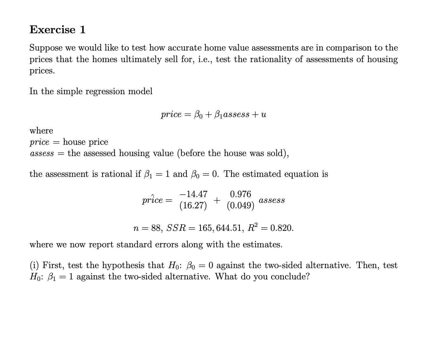
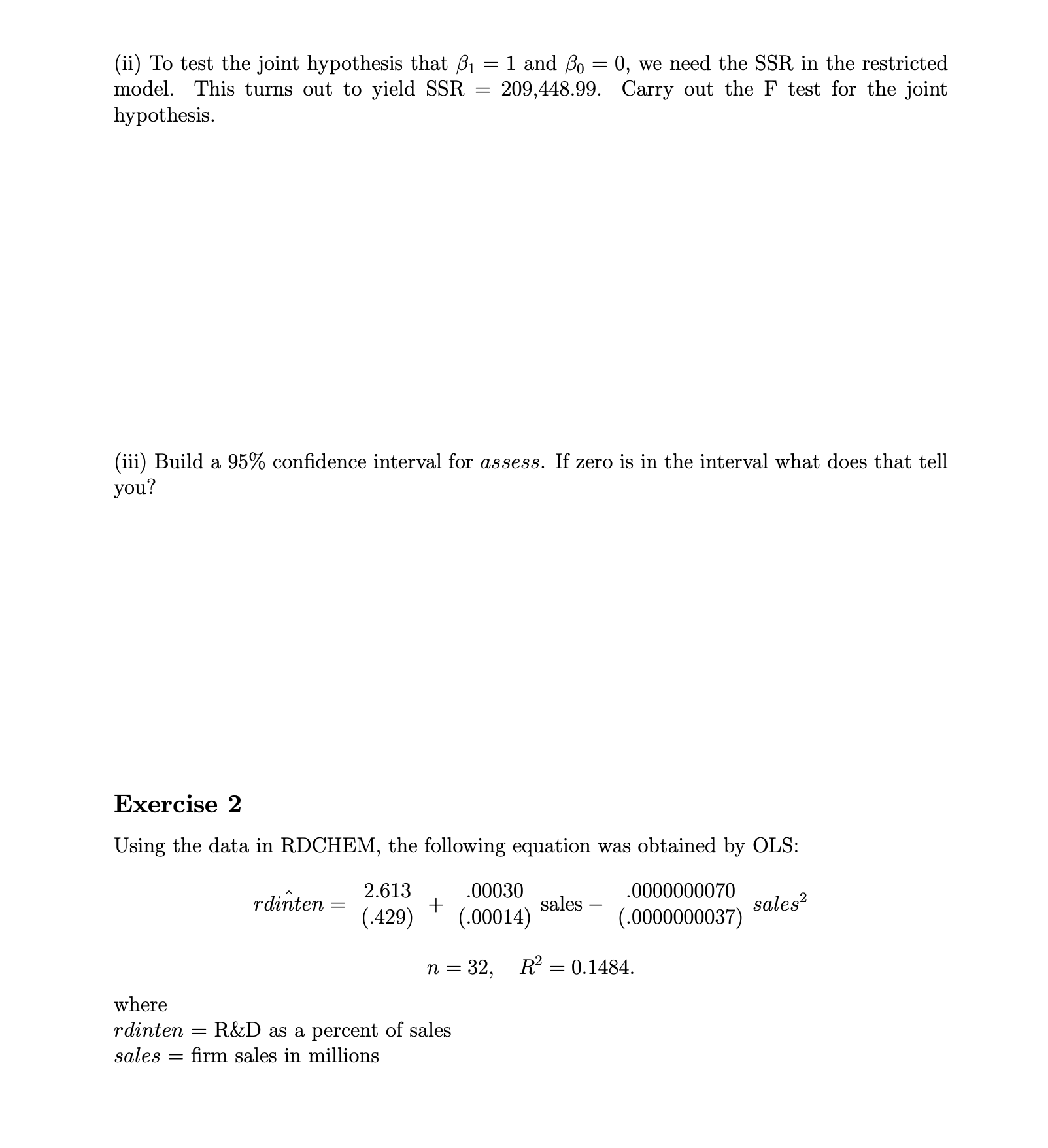
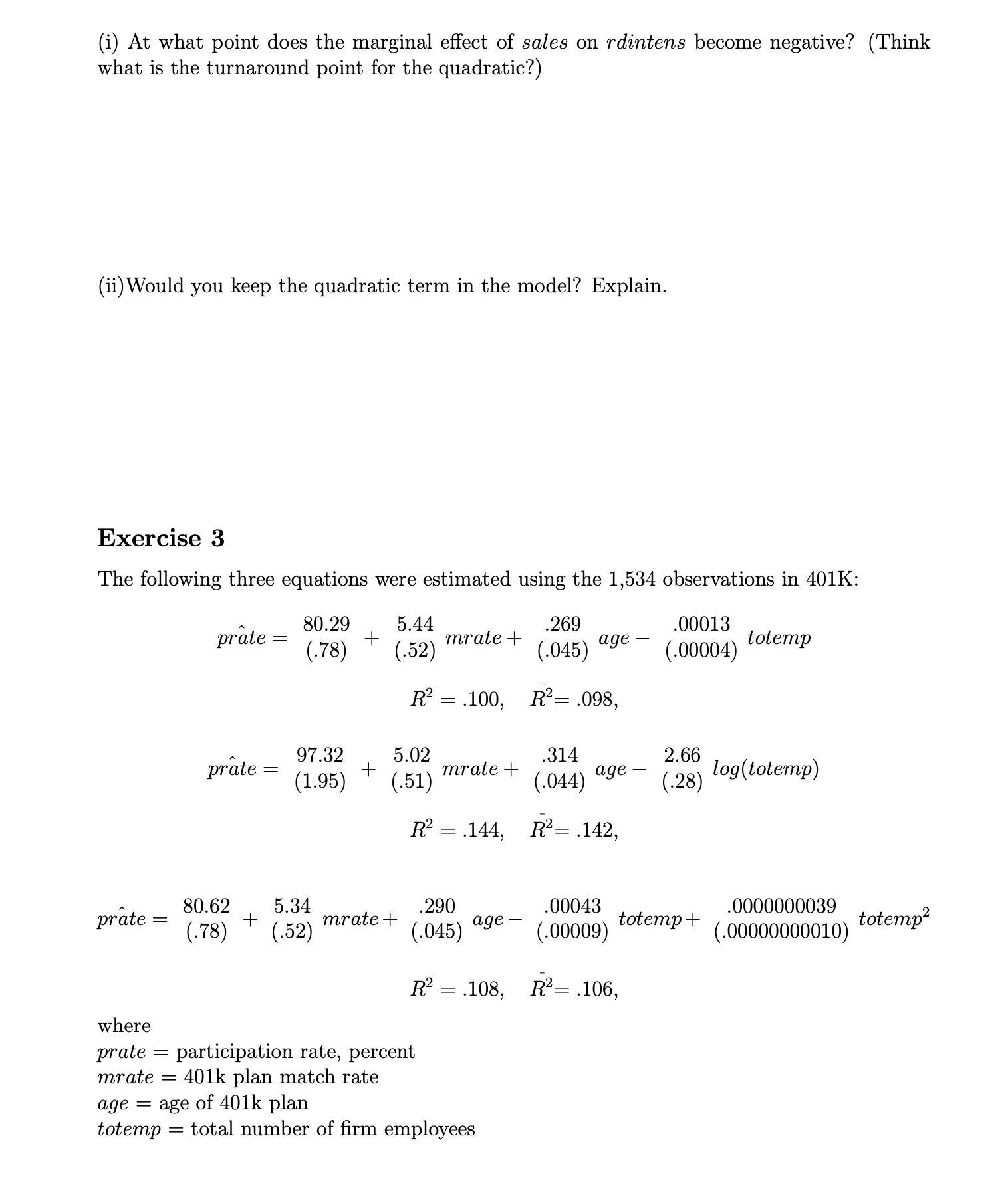
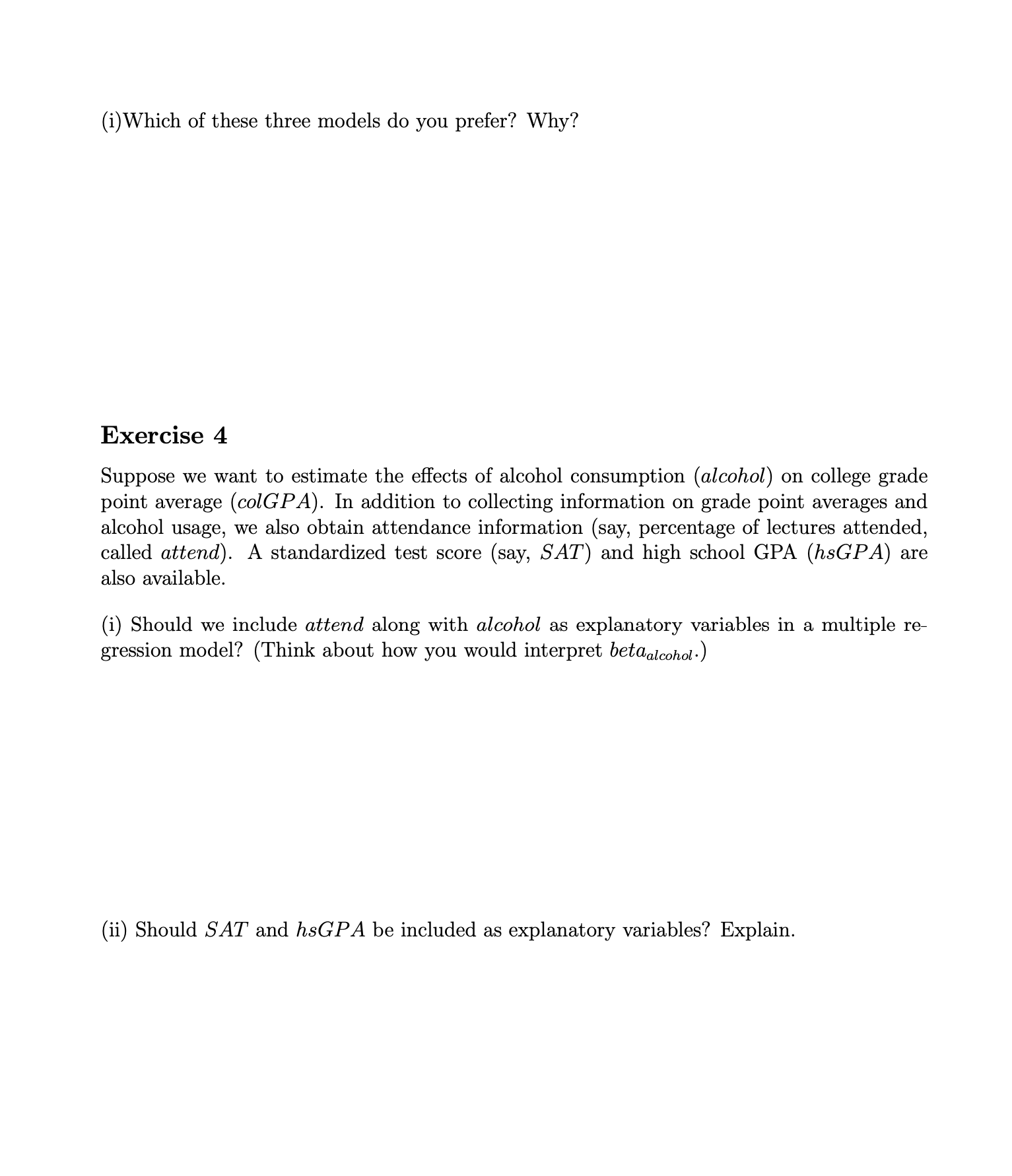
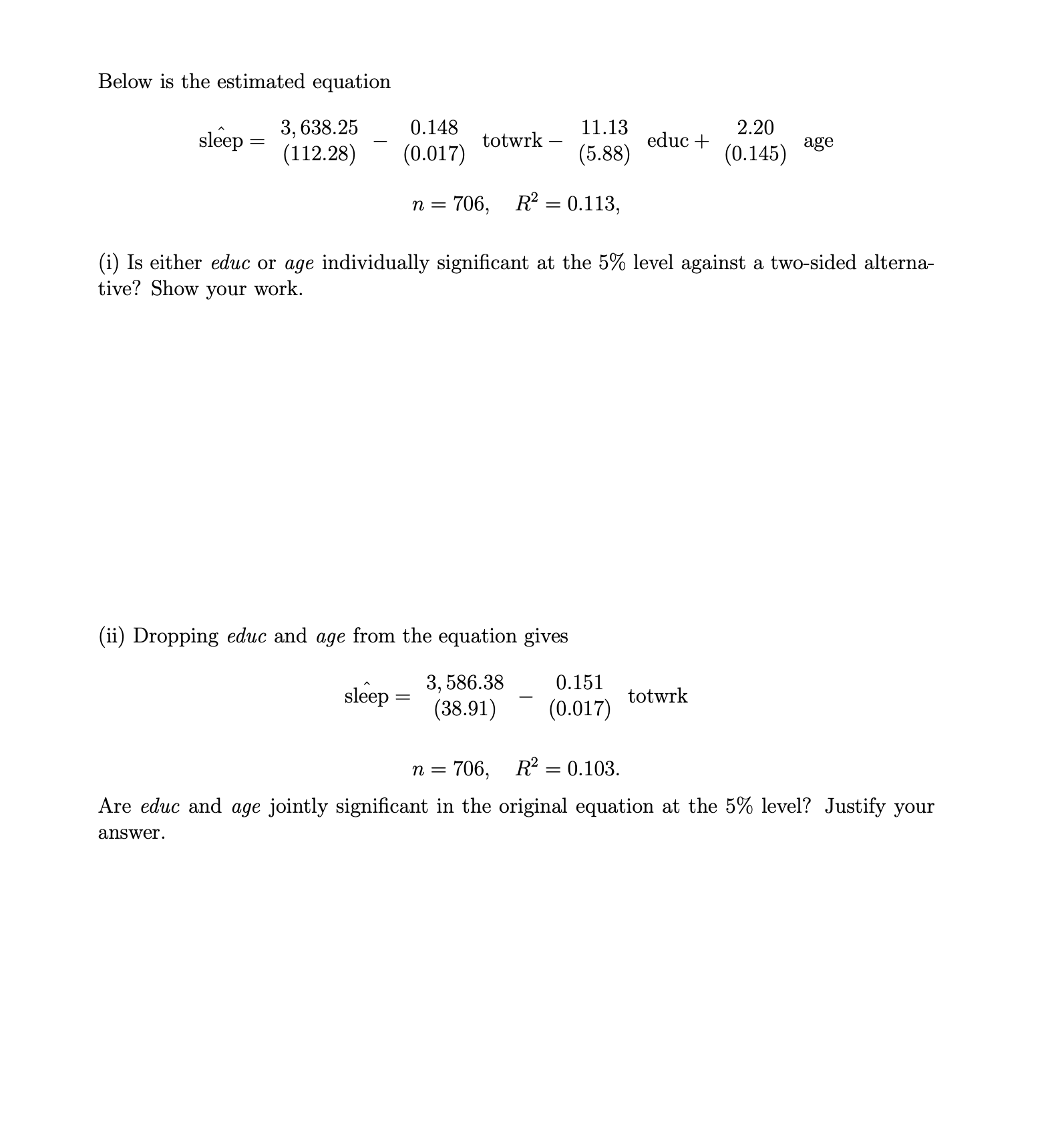
Exercise 1 Suppose we would like to test how accurate home value assessments are in comparison to the prices that the homes ultimately sell for, i.e., test the rationality of assessments of housing prices. In the simple regression model price = By + [Brassess + u where price = house price assess = the assessed housing value (before the house was sold), the assessment is rational if 5, = 1 and By = 0. The estimated equation is 14.47 0.976 (16.27) T (0.049) 2555 price = n = 88, SSR = 165,644.51, R* = 0.820. where we now report standard errors along with the estimates. (i) First, test the hypothesis that Hy: Sy = 0 against the two-sided alternative. Then, test Hy: B1 =1 against the two-sided alternative. What do you conclude? (ii) To test the joint hypothesis that 8; = 1 and 5y = 0, we need the SSR in the restricted model. This turns out to yield SSR = 209,448.99. Carry out the F test for the joint hypothesis. (iii) Build a 95% confidence interval for assess. If zero is in the interval what does that tell you? Exercise 2 Using the data in RDCHEM, the following equation was obtained by OLS: rdinten 2.613 4 .00030 sales .0000000070 sales? (429) T (.00014) (.0000000037) n =32, R?=0.1484. where rdinten = R&D as a percent of sales sales = firm sales in millions (i) At what point does the marginal effect of sales on rdintens become negative? (Think what is the turnaround point for the quadratic?) (ii) Would you keep the quadratic term in the model? Explain. Exercise 3 The following three equations were estimated using the 1,534 observations in 401K: 80.29 5.44 prate = .269 .00013 (.78) + (.52) mrate + (.045) age (.00004) totemp R2 = .100, R2= .098, 97.32 5.02 prate = .314 2.66 (1.95) + (.51) mrate + (.044) age - (.28) log(totemp) R2 = .144, R2= .142, 80.62 5.34 prate = .290 .00043 + mrate + age - totemp+ 0000000039 (.78) (.52) (.045) (.00009) (.00000000010) totemp R2 = .108, R2= .106, where prate = participation rate, percent mrate = 401k plan match rate age = age of 401k plan totemp = total number of firm employees(1)Which of these three models do you prefer? Why? Exercise 4 Suppose we want to estimate the effects of alcohol consumption (alcohol) on college grade point average (colGPA). In addition to collecting information on grade point averages and alcohol usage, we also obtain attendance information (say, percentage of lectures attended, called attend). A standardized test score (say, SAT) and high school GPA (hsGPA) are also available. (1) Should we include attend along with alcohol as explanatory variables in a multiple re- gression model? (Think about how you would interpret beta,iconor-) (ii) Should SAT and hsGPA be included as explanatory variables? Explain. Exercise 5: Stata Use the data in LAWSCH85 for this exercise. The median starting salary for new law school graduates is determined by log(salary) = Bo + BILSAT + B2GPA + Blog(libvol) + BAlog(cost) + Brank + u where LSAT is the median LSAT score for the graduating class, GPA is the median college GPA for the class, libvol is the number of volumes in the law school library, cost is the annual cost of attending law school, and rank is a law school ranking (with rank = 1 being the best). i) Using the model above, state and test the null hypothesis that the rank of law schools has no ceteris paribus effect on median starting salary. (ii) Are features of the incoming class of students-namely, LSAT and GPA-individually or jointly significant for explaining salary?(iii) Test whether the size of the entering class (clsize) or the size of the faculty (faculty) needs to be added to this equation; carry out a single test. (iv) What factors might influence the rank of the law school that are not included in the salary regression? Exercise 6: Stata Use the data in VOTE1 for this exercise. Consider a model with an interaction between expenditures: voteA = Bo + BiprtystrA + ByexpendA + ByexpendB + BA(expendA) * (expendB) + u where voteA = percent vote for A prtystrA = percent vote for president expendA = campaign expenditures by A, $1000s expendB = campaign expenditures by B, $1000si) What is the partial effect of expendB on voteA, holding prtystrA and expendA fixed? What is the partial effect of expendA on voteA? Is the expected sign for beta4 obvious? (ii) Estimate the equation in part (i) and report the results in the usual form. Is the interac- tion term statistically significant? (iii) Find the average of expendA in the sample. Fix expendA at 300 (for $300,000). What is the estimated effect of another $100,000 spent by Candidate B on voteA? Is this a large effect?(iv) Now fix expendB at 100. What is the estimated effect of (expendA) = 100 on voteA? Does this make sense? (v) Now, estimate a model that replaces the interaction with shareA, Candidate A's per- centage share of total campaign expenditures. Does it make sense to hold both expendA and expendB fixed, while changing shareA?Bonus Questions This section is optional and worth up to an extra 10 points on your grade for this problem set, for a possible total of 50/40 points. BONUS: Exercise 7: Stata Use the data in HTV to answer this question. The data set includes information on wages, education, parents' education, and several other variables for 1,230 working men in 1991. where wage = hourly wage abil = ability measure, not standardized motheduc = highest grade completed by mother fatheduc = highest grade completed by father tuitl7 = college tuition, age 17 tuitl8 = college tuition, age 18 (i) Estimate the regression model educ = By + fimotheduc + B2 fatheduc + Bzabil + Biabil +u by OLS and report the results in the usual form. Test the null hypothesis that educ is linearly related to abil against the alternative that the relationship is quadratic. (ii) Using the equation in part (i), test Hy: 1 = (o against a two-sided alternative. What is the p-value of the test? (iii) Add the two college tuition variables to the regression from part (i) and determine whether they are jointly statistically significant. BONUS: Exercise 8 The following model is a simplified version of the multiple regression model used by Biddle and Hamermesh (1990) to study the tradeoff between time spent sleeping and working and to look at other factors affecting sleep: sleep = By + Prtotwrk + Paeduc + Psage + u, where sleep and totwrk (total work) are measured in minutes per week and educ and age are measured in years. Below is the estimated equation ~ 3,638.25 0.148 11.13 2.20 sleep = totwrk educ + (0.145) (112.28) (0.017) (5.88) age n =706, R?'=0.113, (i) Is either educ or age individually significant at the 5% level against a two-sided alterna- tive? Show your work. (ii) Dropping educ and age from the equation gives 3,586.38 0.151 (38.91) ~ (0.017) Ok slep = n =706, R?=0.103. Are educ and age jointly significant in the original equation at the 5% level? Justify your answer. (iii) Does including educ and age in the model greatly affect the estimated tradeoff between sleeping and working