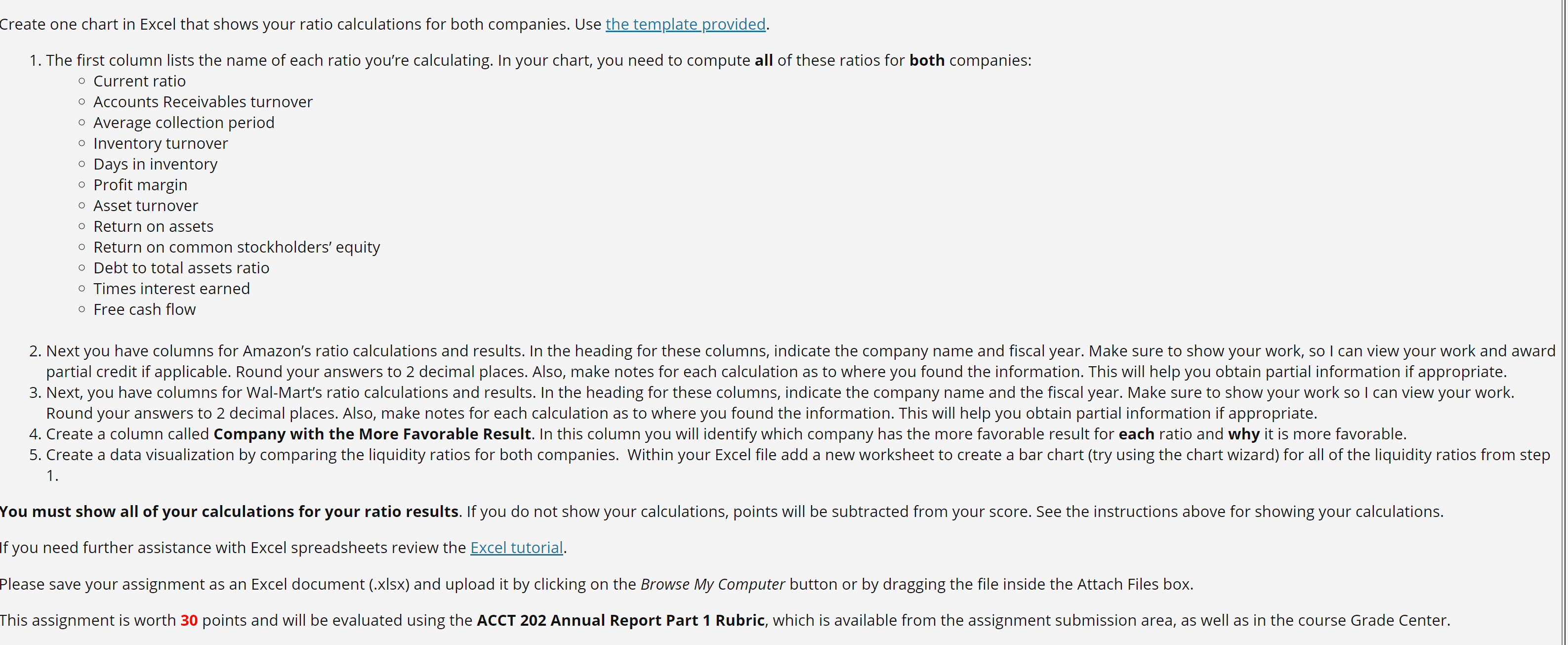
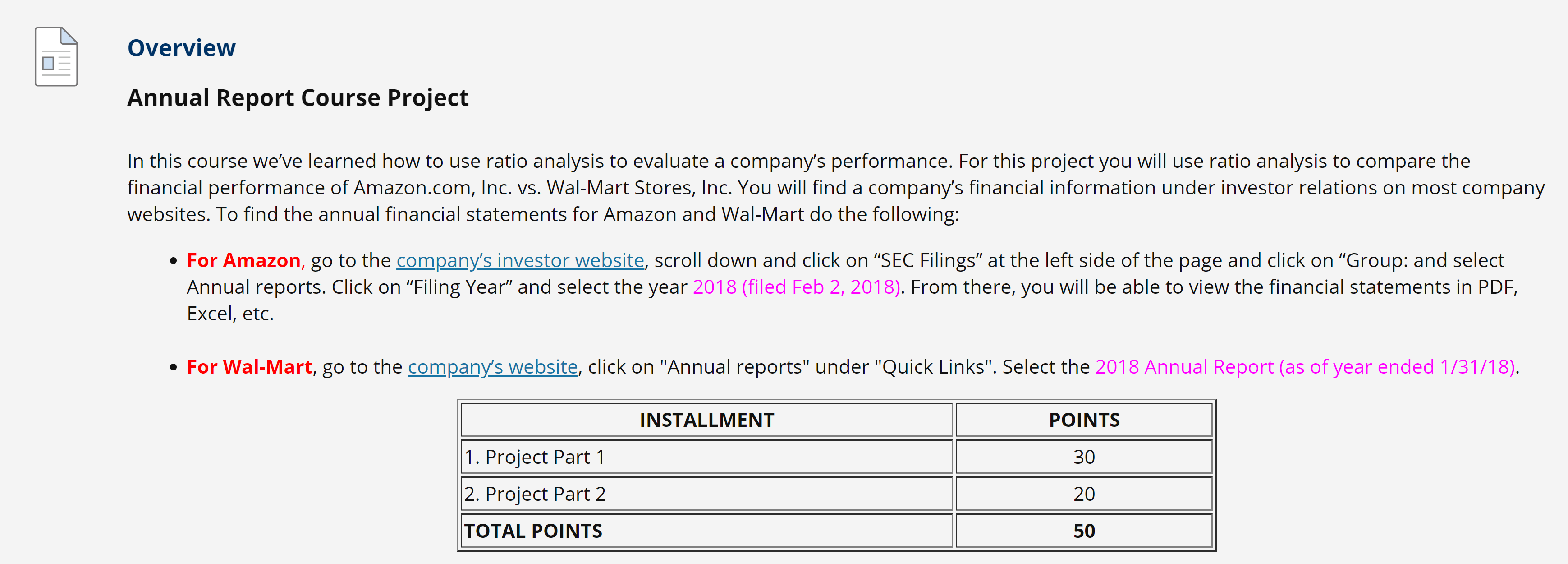
Create one chart in Excel that shows your ratio calculations for both companies. Use the template provided. 1 . The first column lists the name of each ratio you're calculating. In your chart, you need to compute all of these ratios for both companies: o o o o o o o Current ratio Accounts Receivables turnover Average collection period Inventory turnover Days in inventory Profit margin Asset turnover Return on assets Return on common stockholders' equity Debt to total assets ratio Times interest earned Free cash flow 2. Next you have columns for Amazon's ratio calculations and results. In the heading for these columns, indicate the company name and fiscal year. Make sure to show your work, so I can view your work and award partial credit if applicable. Round your answers to 2 decimal places. Also, make notes for each calculation as to where you found the information. This will help you obtain partial information if appropriate. 3. Next, you have columns for Wal-Mart's ratio calculations and results. In the heading for these columns, indicate the company name and the fiscal year. Make sure to show your work so I can view your work. Round your answers to 2 decimal places. Also, make notes for each calculation as to where you found the information. This will help you obtain partial information if appropriate. 4. Create a column called Company with the More Favorable Result. In this column you will identify which company has the more favorable result for each ratio and why it is more favorable. 5. Create a data visualization by comparing the liquidity ratios for both companies. Within your Excel file add a new worksheet to create a bar chart (try using the chart wizard) for all of the liquidity ratios from step You must show all of your calculations for your ratio results. If you do not show your calculations, points will be subtracted from your score. See the instructions above for showing your calculations. If you need further assistance with Excel spreadsheets review the Excel tutorial. Please save your assignment as an Excel document (.xlsx) and upload it by clicking on the Browse My Computer button or by dragging the file inside the Attach Files box. This assignment is worth 30 points and will be evaluated using the ACCT 202 Annual Report Part 1 Rubric, which is available from the assignment submission area, as well as in the course Grade Center.