fill in the blanks and make a spreadsheet for section 2&3

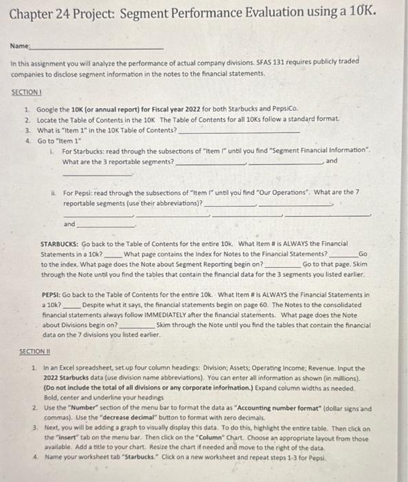
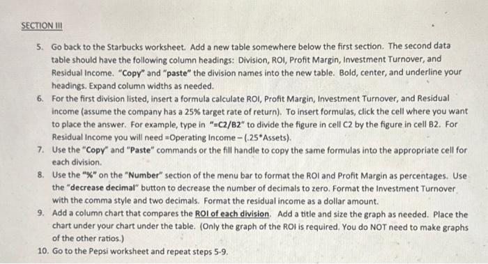
Chapter 24 Project: Segment Performance Evaluation using a 10K. Name: In this assignment you will analyze the performance of actual company divisions. SFAS 131 requires publicly traded companies to disclose segment information in the notes to the financial statements. SECTIONI 1. Google the 10K (or annual report) for Fiscal year 2022 for both Starbucks and Pepsico. 2. tocate the Table of Contents in the 10K. The Table of Contents for all 1OKs follow a standard format. 3. What is "Item 1 " in the 10K Table of Contents? 4. Go to "Item 1" 1. For Starbucks: read through the subsections of "Item I" until you find "Segment Financial Information". What are the 3 reportable segments? and reportable segments (use their abbreviations)? and STARBUCKS: Go back to the Table of Contents for the entire 10K. What item $ is ALWAYS the Financial Statements in a 10k ? What page contains the Index for Notes to the Financial Statements? Go to the index. What page does the Note about Segment Reporting begin on? Go to that page, Skim through the Note untli you find the tables that contain the financial data for the 3 segments you listed earlier. PEPSI: Go back to the Table of Contents for the entire 10k. What Item \# is ALWAYS the Financial Statements in a 10k ? Despite what it says, the financial statements begin on page 60 . The Notes to the consolidated financial statements always follow IMMEDLATELY after the financial statements. What page does the Note about Divisions begin on? Skim through the Note until you find the tables that contain the financial data on the 7 divisions you listed earlier. SECTION II 1. In an Excel spreadsheet, setup four column headings: Division; Assets; Operating income; Revenue. Input the 2022 starbucks data (use division name abbreviations). You can enter all information as shown (in millions). (Do not include the total of all divisions or any corporate inforination.) Expand column widths as needed. Bold, center and underline your headings 2. Use the "Number" section of the menu bar to format the data as "Accounting number format" (dollar signs and commas). Use the "decrease decimal" button to format with zero decimals. 3. Next, you will be adding a graph to visually display this data. To do this, highlight the entire table. Then click on the "insert" tab on the menu bar. Then click on the "Column" Chart. Choose an appropriate layout from those available. Add a title to your chart. Resize the chart if needed and move to the right of the data. 4. Name your worksheet tab "starbucks." Click on a new worksheet and repeat steps 1-3 for Pepsi. SECTION III 5. Go back to the Starbucks worksheet. Add a new table somewhere below the first section. The second data table should have the following column headings: Division, ROI, Profit Margin, Investment Turnover, and Residual Income. "Copy" and "paste" the division names into the new table. Bold, center, and underline your headings. Expand column widths as needed. 6. For the first division listed, insert a formula calculate ROI, Profit Margin, Investment Turnover, and Residual income (assume the company has a 25% target rate of return). To insert formulas, click the cell where you want to place the answer. For example, type in " =C2/B2 " to divide the figure in cell C2 by the figure in cell B2. For Residual Income you will need = Operating Income (.25 Assets) . 7. Use the "Copy" and "Paste" commands or the fill handle to copy the same formulas into the appropriate cell for each division. 8. Use the "\%" on the "Number" section of the menu bar to format the ROI and Profit Margin as percentages. Use the "decrease decimal" button to decrease the number of decimals to zero. Format the Investment Turnover with the comma style and two decimals. Format the residual income as a dollar amount. 9. Add a column chart that compares the ROI of each division. Add a title and size the graph as needed. Place the chart under your chart under the table. (Only the graph of the ROI is required, You do NOT need to make graphs of the other ratios.) 10. Go to the Pepsi worksheet and repeat steps 5-9