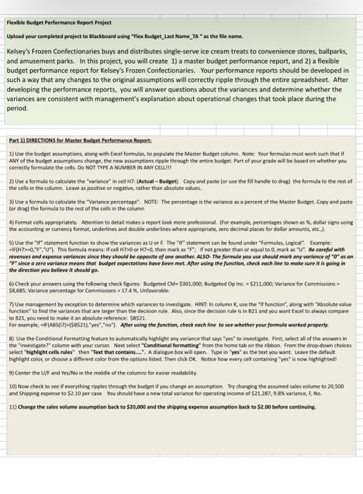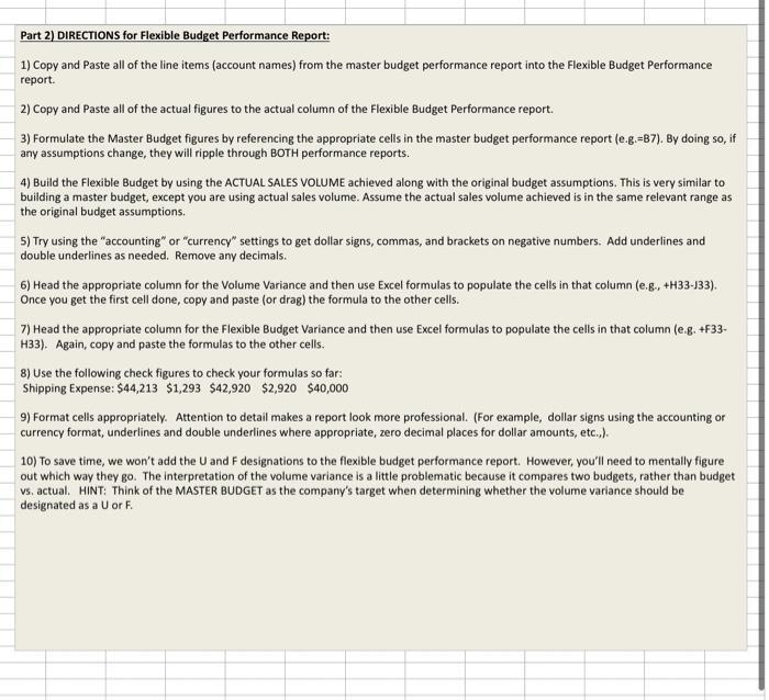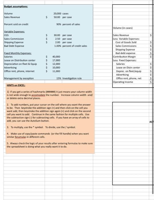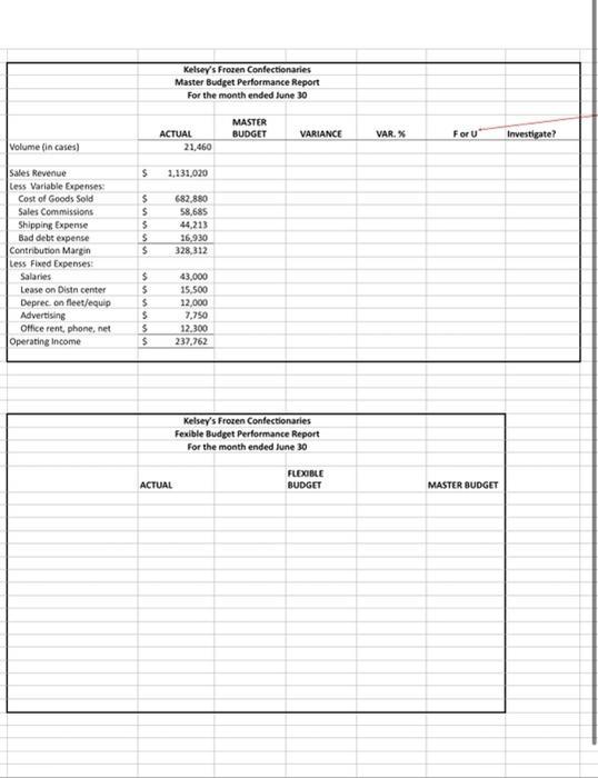
Flexible Budget Performance Report Project Upload your completed project to Blackboard using "Flex Budget_Last Name_TA " as the file name. Kelsey's Frozen Confectionaries buys and distributes single-serve ice cream treats to comvenience stores, ballparks, and amusement parks. In this project, you will create 1) a master budget performance report, and 2) a flexible budget performance report for Kelsey's Frozen Confectionaries. Your performance reports should be developed in such a way that any changes to the original assumptions will correctly ripple through the entire spreadsheet. After developing the performance reports, you will answer questions about the variances and determine whether the variances are consistent with management's explanation about operational changes that took place during the period. Part 1) DIRECTIONS for Master Budget Performance Repart 1) Use the budget assumptions, along with Ixcel formulas, to populate the Master Budget column. Note: Your formulas must work such that if ANY of the budget assumptions change, the new assumptions ripple through the entire budget. Part ef your srade will be based an whether you coerectly formulate the cels. Do NOT TYPE A NUMIER IN ANY CELLII! 2) Use a formula to calculate the "variance" in cell H7: (Actual - Budget). Copy and paste (or use the fill handle to drag) the formula to the rest of the cells in the column, Leare as positive or negative, rather than absolute values. 3) Use a formula to calculste the "Variance persentage". NoTe. The percentage is the variance as a percent of the Master Budget. Copy and paste (or drag) the formula to the rest of the ceils in the column 4) Format cells appropriately Attention to detail makes a report look more professional. (For example, percentages shown as % dollar signs using, the accounting or currency format, underines and double underines where appeopriate, zero decimal places for dollar amounts, etc., 5) Use the "If" statement function to show the variances as U or E. The " A " statement can be found under "Formulas, Logical", Example: revenues and expense varionces siace they should be opposite of ane another. Also. The farmulo you use should mark any variance of "o" as an "F" since a rero variance means that budget expectations have been met. After asing the function, check each fine to make sure it is going in the direction you belleve it should go. 6) Check your answers using the following check figures. Badgeted CM=$301.000, Budgeted 0p inc: =$211,000; Variance for Commissions = \$8,685, Variance percentage for Commissions =17,4%, Unfevorable. 7) Use management by exception to determine which variances to investigate. HINT: In column K, use the "If function", along with "Absolute value function" to find the variances that are larger than the deckion rule. Aso, since the decision rule is in B21 and you want Ercel to always compare. to B21, you need to make is an absolute reference. 58521 . For example, =if(AB5117)>\{SBS21), "Yes", "no"]. After using the function, check eoch fine to see whether your formula warked properly. 8) Use the Conditional Formatting feature to automatically highlyent any variance that qys "yes" to investigate. First, select all of the answers in the "investigate?" column with your cursor. Neat select "Conditional formatting" from the home tab on the ribbon. From the drop dowa choices select "highlight cells rules" then "Text that contains...". A dialogue bax will open. Type in "yes" as the teas you want. Leave the defaul highlight color, or choose a different color from the options lsted. Then dick OK. Notice how every cell containing "yes" is now highighted 9) Center the U/F and Yes/No in the middle of the columns for easier readability. 10) Now check to see if everything ripples through the budget if you change an ascumption. Try changing the assumed sales volume to 20 , 500 and Shipping expense to $2.10 per case. You should have a new total variance for operating income of $21,287,9.8% variance, F, No. 11) Change the sales volume assumption back to $20,000 and the shipping expense assumption back to $2.00 before continuing. Part 2) DIRECTIONS for Flexible Budget Performance Report: 1) Copy and Paste all of the line items (account names) from the master budget performance report into the Flexible Budget Performance report. 2) Copy and Paste all of the actual figures to the actual column of the Flexible Budget Performance report. 3) Formulate the Master Budget figures by referencing the appropriate cells in the master budget performance report (e.g. =87 ). By doing so, if any assumptions change, they will ripple through BOTH performance reports. 4) Build the Flexible Budget by using the ACTUAL SALES VOLUME achieved along with the original budget assumptions. This is very similar to building a master budget, except you are using actual sales volume. Assume the actual sales volume achieved is in the same relevant range as the original budget assumptions. 5) Try using the "accounting" or "currency" settings to get dollar signs, commas, and brackets on negative numbers. Add underlines and double underlines as needed. Remove any decimals. 6) Head the appropriate column for the Volume Variance and then use Excel formulas to populate the cells in that column (e.g., +H33J33 ). Once you get the first cell done, copy and paste (or drag) the formula to the other cells. 7) Head the appropriate column for the Flexible Budget Variance and then use Excel formulas to populate the cells in that column (e.g. + F33H33). Again, copy and paste the formulas to the other cells. 8) Use the following check figures to check your formulas so far: Shipping Expense: $44,213$1,293$42,920$2,920$40,000 9) Format cells appropriately. Attention to detail makes a report look more professional. (For example, dollar signs using the accounting or currency format, underlines and double underlines where appropriate, zero decimal places for dollar amounts, etc.,). 10) To save time, we won't add the U and F designations to the flexible budget performance report. However, you'll need to mentally figure out which way they go. The interpretation of the volume variance is a little problematic because it compares two budgets, rather than budget vs. actual. HINT: Think of the MASTER BUDGET as the company's target when determining whether the volume variance should be designated as a U or F. HINTS On EXCFL: 1) If you get a series of hashmarks (Hanaza) it just means your column width is not wide enough to ackomodate the number. Increase column width and/ or delete extra decimal places. 2. To add numbers, put your cursor on the cell where you want the answer to be. Then keystroke the addition sign (t) and then click on the cell you want add, then keystroke the addition sign again (t) and dick on the second cell you want to add. Continue in the same fashion for multiple cells. Use the subtraction sign ( ) for subtracting cells. If you have an array of cells to add, you can use the Autosum button. 3. To multiply, use the * symbol. To divide, use the / symbol. 4. Make use of copy/paste commands (or the fill handle) when you want similar forumulas in different cells. 5. Always check the logic of your results after enteting formulas to make sure the spreadsheet is doing what you really want it to do. Kelsey's Frosen Confectionaries Fexible Budget Performance Report For the mooth ended lune 30 Flexible Budget Performance Report Project Upload your completed project to Blackboard using "Flex Budget_Last Name_TA " as the file name. Kelsey's Frozen Confectionaries buys and distributes single-serve ice cream treats to comvenience stores, ballparks, and amusement parks. In this project, you will create 1) a master budget performance report, and 2) a flexible budget performance report for Kelsey's Frozen Confectionaries. Your performance reports should be developed in such a way that any changes to the original assumptions will correctly ripple through the entire spreadsheet. After developing the performance reports, you will answer questions about the variances and determine whether the variances are consistent with management's explanation about operational changes that took place during the period. Part 1) DIRECTIONS for Master Budget Performance Repart 1) Use the budget assumptions, along with Ixcel formulas, to populate the Master Budget column. Note: Your formulas must work such that if ANY of the budget assumptions change, the new assumptions ripple through the entire budget. Part ef your srade will be based an whether you coerectly formulate the cels. Do NOT TYPE A NUMIER IN ANY CELLII! 2) Use a formula to calculate the "variance" in cell H7: (Actual - Budget). Copy and paste (or use the fill handle to drag) the formula to the rest of the cells in the column, Leare as positive or negative, rather than absolute values. 3) Use a formula to calculste the "Variance persentage". NoTe. The percentage is the variance as a percent of the Master Budget. Copy and paste (or drag) the formula to the rest of the ceils in the column 4) Format cells appropriately Attention to detail makes a report look more professional. (For example, percentages shown as % dollar signs using, the accounting or currency format, underines and double underines where appeopriate, zero decimal places for dollar amounts, etc., 5) Use the "If" statement function to show the variances as U or E. The " A " statement can be found under "Formulas, Logical", Example: revenues and expense varionces siace they should be opposite of ane another. Also. The farmulo you use should mark any variance of "o" as an "F" since a rero variance means that budget expectations have been met. After asing the function, check each fine to make sure it is going in the direction you belleve it should go. 6) Check your answers using the following check figures. Badgeted CM=$301.000, Budgeted 0p inc: =$211,000; Variance for Commissions = \$8,685, Variance percentage for Commissions =17,4%, Unfevorable. 7) Use management by exception to determine which variances to investigate. HINT: In column K, use the "If function", along with "Absolute value function" to find the variances that are larger than the deckion rule. Aso, since the decision rule is in B21 and you want Ercel to always compare. to B21, you need to make is an absolute reference. 58521 . For example, =if(AB5117)>\{SBS21), "Yes", "no"]. After using the function, check eoch fine to see whether your formula warked properly. 8) Use the Conditional Formatting feature to automatically highlyent any variance that qys "yes" to investigate. First, select all of the answers in the "investigate?" column with your cursor. Neat select "Conditional formatting" from the home tab on the ribbon. From the drop dowa choices select "highlight cells rules" then "Text that contains...". A dialogue bax will open. Type in "yes" as the teas you want. Leave the defaul highlight color, or choose a different color from the options lsted. Then dick OK. Notice how every cell containing "yes" is now highighted 9) Center the U/F and Yes/No in the middle of the columns for easier readability. 10) Now check to see if everything ripples through the budget if you change an ascumption. Try changing the assumed sales volume to 20 , 500 and Shipping expense to $2.10 per case. You should have a new total variance for operating income of $21,287,9.8% variance, F, No. 11) Change the sales volume assumption back to $20,000 and the shipping expense assumption back to $2.00 before continuing. Part 2) DIRECTIONS for Flexible Budget Performance Report: 1) Copy and Paste all of the line items (account names) from the master budget performance report into the Flexible Budget Performance report. 2) Copy and Paste all of the actual figures to the actual column of the Flexible Budget Performance report. 3) Formulate the Master Budget figures by referencing the appropriate cells in the master budget performance report (e.g. =87 ). By doing so, if any assumptions change, they will ripple through BOTH performance reports. 4) Build the Flexible Budget by using the ACTUAL SALES VOLUME achieved along with the original budget assumptions. This is very similar to building a master budget, except you are using actual sales volume. Assume the actual sales volume achieved is in the same relevant range as the original budget assumptions. 5) Try using the "accounting" or "currency" settings to get dollar signs, commas, and brackets on negative numbers. Add underlines and double underlines as needed. Remove any decimals. 6) Head the appropriate column for the Volume Variance and then use Excel formulas to populate the cells in that column (e.g., +H33J33 ). Once you get the first cell done, copy and paste (or drag) the formula to the other cells. 7) Head the appropriate column for the Flexible Budget Variance and then use Excel formulas to populate the cells in that column (e.g. + F33H33). Again, copy and paste the formulas to the other cells. 8) Use the following check figures to check your formulas so far: Shipping Expense: $44,213$1,293$42,920$2,920$40,000 9) Format cells appropriately. Attention to detail makes a report look more professional. (For example, dollar signs using the accounting or currency format, underlines and double underlines where appropriate, zero decimal places for dollar amounts, etc.,). 10) To save time, we won't add the U and F designations to the flexible budget performance report. However, you'll need to mentally figure out which way they go. The interpretation of the volume variance is a little problematic because it compares two budgets, rather than budget vs. actual. HINT: Think of the MASTER BUDGET as the company's target when determining whether the volume variance should be designated as a U or F. HINTS On EXCFL: 1) If you get a series of hashmarks (Hanaza) it just means your column width is not wide enough to ackomodate the number. Increase column width and/ or delete extra decimal places. 2. To add numbers, put your cursor on the cell where you want the answer to be. Then keystroke the addition sign (t) and then click on the cell you want add, then keystroke the addition sign again (t) and dick on the second cell you want to add. Continue in the same fashion for multiple cells. Use the subtraction sign ( ) for subtracting cells. If you have an array of cells to add, you can use the Autosum button. 3. To multiply, use the * symbol. To divide, use the / symbol. 4. Make use of copy/paste commands (or the fill handle) when you want similar forumulas in different cells. 5. Always check the logic of your results after enteting formulas to make sure the spreadsheet is doing what you really want it to do. Kelsey's Frosen Confectionaries Fexible Budget Performance Report For the mooth ended lune 30