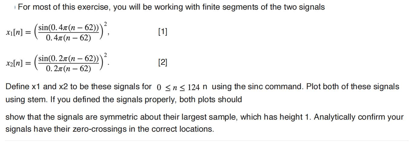
For most of this exercise, you will be working with finite segments of the two signals (sin(0.47 (n 62))) - 0.4(n-62) x[n] = x[n]: (sin(0.27 (n = 62))) . - [1] [2] Define x1 and x2 to be these signals for 0 n 124 n using the sinc command. Plot both of these signals using stem. If you defined the signals properly, both plots should show that the signals are symmetric about their largest sample, which has height 1. Analytically confirm your signals have their zero-crossings in the correct locations. (b) Analytically compute the DTFTs X(e) and X(e) of x[n] and x[n] as given in Eqs. (1) and (2), ignoring the effect of truncating the signals. k Use fft to compute the samples of the DTFT of the truncated signals in x1 and x2 at wk = 2 2048 for 0 k 2047 and store the results in X1 and X2. Generate appropriately labeled plots of the magnitudes of X1 and X2. How do these plots compare with your analytical expressions? xe[n]: {:1 0 n = k L, k integer otherwise If x is a row vector containing x[n], the following commands implement expanding by L >> xe = zeros (1, L*length(x)); >> xe(1:L:length(xe)) = X; Based on this template, define xe1 and xe2 to be x1 and x2 expanded by a factor of 3. Also, define Xe1 and Xe2 to be 2048 samples of the DTFT of these expanded signals computed using fft. Generate appropriately labeled plots of the magnitude of these DTFTs. Expanding by L should give a DTFT X(ei). Do your plots agree with this? Note: If you want to increase the sampling rate by L, you need to interpolate between the samples of xe[n] with a lowpass filter with cutoff frequency wc = This filter will remove the compressed copies of X(e) T L E, except the ones centered at @c = 2k. The resulting spectrum is that which would have been L located every obtained if the original bandlimited continuous-time signal had been sampled L times faster. For this reason, the combination of expansion and interpolation is often referred to as upsampling a signal. (d) If the row vector x contains the signal x[n], the following MATLAB command will implement downsampling by an integer factor M >> xd = x (1 : M: length(x)); Based on the DTFTs you found analytically in Part (b), state for both x[n] and x[n] if the signal can be downsampled by a factor of 2 without introducing aliasing. If downsampling introduces aliasing, indicate which frequencies are corrupted by the aliasing and which are not affected. If the signal can be downsampled without introducing aliasing, sketch the magnitude of X(e"), the DTFT of downsampledsignal. (e) Define xd1 and xd2 to be the result of downsampling x1 and x2 by 2. Define Xd1 and Xd2 to be samples of the DTFTs of the downsampled signals computed at 2048 evenly spaced samples between 0 and 2. Generate appropriately labeled plots of the magnitudes of both DTFTs. Do the plots agree with your sketch(es) from Part (d)?